Moveout-based wave-equation migration velocity analysis

Results

We create several synthetic examples to show the effectiveness of our method. The model is 16km in x and 1.2km in z. The grid sampling is 20m in x and 10m in z. The survey geometry follows the marine acquisition convention with 4km cable length, receiver spacing is 20m and a total of 150 shots are simulated from -6km to +6km with a spacing of 80m. A total of 106 frequencies are calculated, ranging from 5Hz to 40Hz. Unless explicitly mentioned, there is one flat reflector at a depth around 800m and a constant background velocity of 2000m/s is used. A one-way propagator is used for computational efficiency. For comparison, the subsurface-offset DSO and straight maximum-stack-power method are also implemented.

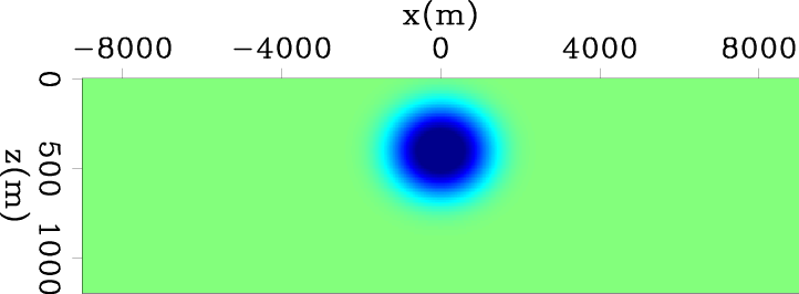
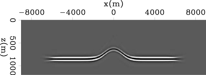
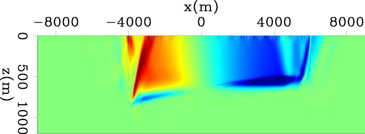
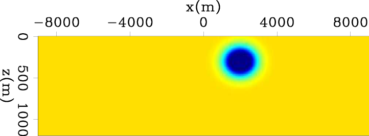
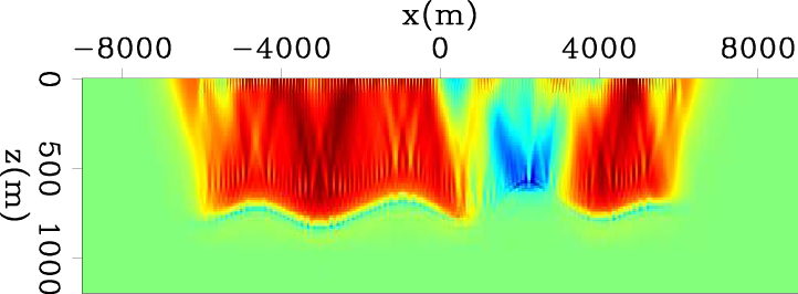
The first example is a true velocity with a 1km width Gaussian anomaly at the center, with peak value 4000m/s. Figure 3(a) shows the anomaly (in slowness) and Fig 3(b) shows the migrated zero subsurface-offset image, The velocity error is so large that the center part of the reflector is pulled up significantly.

vel2.a5,img21w.a5.0off
Figure 3. (a) The slowness model with a Gaussian anomaly.(b) The migrated image using constant background slowness.

dS21w.a5.bf2g,dS21w.a5.dso,dS21w.a5.1
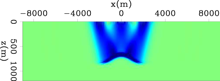
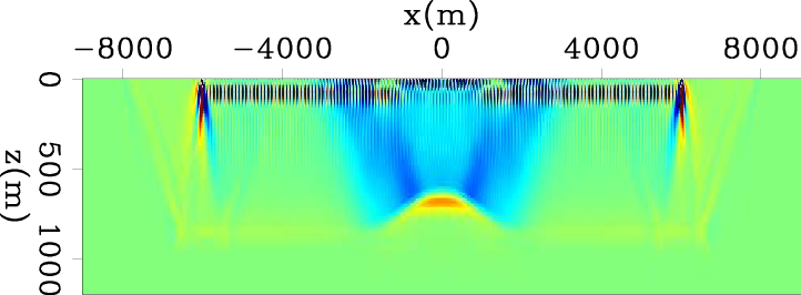
Figure 4. The first slowness update direction of our method (a), the subsurface-offset domain DSO (b), and the direct stack-power-maximization (c), true slowness refers to figure 3(a).

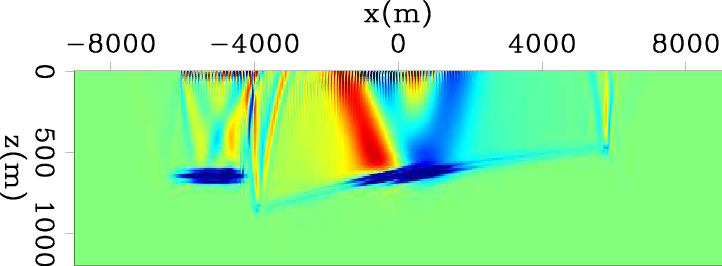
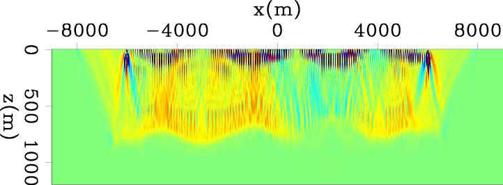
Figure 4 shows the first slowness update using the three methods. Our method presents the most pleasing update among the three; the location of the anomaly is correctly located, and the target region is more uniformly updated, except for the small holes within the ``W'' shape due to the poorer wave path coverage caused by the curved reflector. The DSO result shows the typical strip-shaped artifacts, and the amplitude of the target region is weak compared to the edge artifacts. The maximum-stack-power method suffers from cycle skipping and is not able to locate the target area.

vel2.hg,img21w.hg.0off
Figure 5. (a) The slowness model with a horizontal gradient from 1500m/s to 2700m/s ;(b) The migrated image using constant background slowness.

dS21w.hg.bf2g,dS21w.hg.dso,dS21w.hg.1
Figure 6. The first slowness update direction of our method (a), the subsurface-offset domain DSO (b), and direct stack power maximization (c). The true slowness refers to figure 5(a).

In the second example the true velocity has a horizontal gradient, where velocity increase linearly from 1500 m/s to 2700 m/s. Figure 5(a) shows the true model (in slowness) and figure 5(b) shows the migrated zero subsurface-offset image. The originally flat reflector is tilted in the image because of the horizontal slowness gradient.

Figure 6 shows the first slowness update using the three methods. Again our method presents the most pleasing update among the three. The amplitude of the search direction is proportional to the actual magnitude of the slowness error. A large strip-shaped artifact is introduced at $x=-4000\,m$ in DSO update. this is commonly seen from DSO results when there are reflector discontinuities; although it does decently predicted the horizontal gradient shape of the slowness error. The maximum-stack-power method is able to predict correctly when the slowness error is small (around $x=0\,m$ ). As the slowness error reaches a certain threshold, cycle-skipping happens and the result deteriorates.

vel2.bump,img21w.bump.0off,dS21w.bump.bf2g,dS21w.bump.dso
Figure 7. (a) The slowness model with a constant slower velocity $1900\,m/s$ , there is also a high velocity anomaly at $x=2000\,m$ , with peak value $2850\,m/s$ ; (b) The migrated image using constant background velocity ($2000\,m/s$ ). (c) The first slowness update direction using our method; (d) The first slowness update using the subsurface-offset domain DSO method.

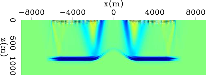
For the third example, the true velocity is a constant $1900\,m/s$ plus a high veloicty anomaly at $x=2000\,m/s$ with peak value $2850\,m/s$ . We designed a hump-shaped reflector to test this method's ability to handle mild dips. Figure 7(a) shows the true model (in slowness) and Fig 7(b) shows the migrated zero subsurface-offset image. Figure 7(c) and 7(d) shows the first slowness update using our method and the DSO method. The effect of the high velocity anomaly is partially cancelled by the lower constant part ($1900\,m/s$ ), nontheless, the overall result still requires a negative update at the anomaly's location. In the presence of a mild dipping reflector, our method still yields a satisfying result.

The effect of the high velocity anomaly is partially cancelled by the lower constant part ($1900\,m/s$ ), nontheless, the overall result still requires a negative update at the anomaly's location. In the presence of a mild dipping reflector, our method still yields a satisfying result.

v.sm.marm,v.zg.marm,vinv.zg.bf2g.marm,vinv.zg.dso.marm
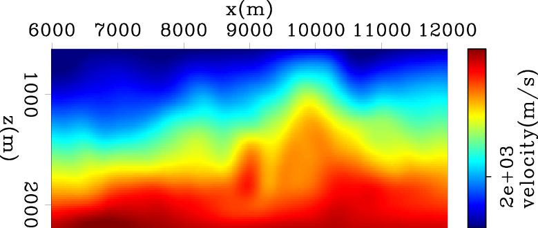
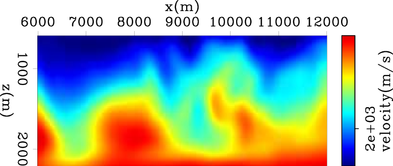
Figure 8. The true velocity model of Marmousi (a) (slightly smoothed) ; the starting velocity model (b) ; the inverted velocity model using our method (c) and using the subsurface-offset DSO (d).

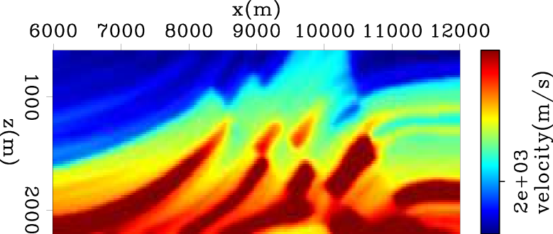
Based on the gradient calculation, we implement an non-linear slowness inversion framework. The example we tested is the marmousi velocity model. The model is $6\,km$ in x and $1.6\,km$ in z. The spatial sampling is $20\,m$ . The survey geometry follows the land acquisition convention with receiver at every surface location on the top and a total of 51 shots are simulated covering the whole lateral span on the top with a spacing of $120\,m$ .

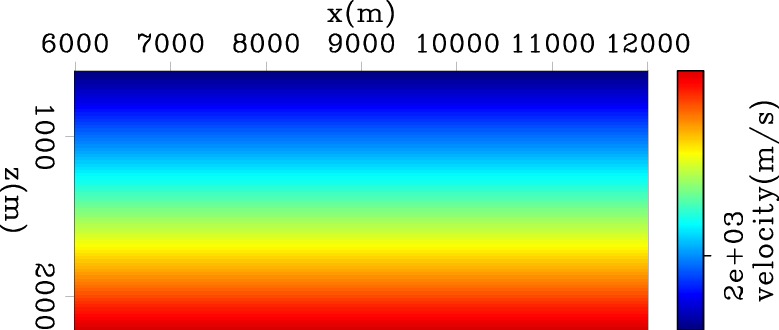
Figure 8(a) shows the true model (in velocity) and figure 8(b) shows the starting model, which has a vertical gradient increasing from $1600\,m/s$    to $3200\,m/s$ . Figure 8(c) and 8(d) show the inverted velocity model using our method and subsurface-offset DSO method. We run 20 nonlinear iterations for each inversion, and the same extent of gradient smoothing is applied. Although both inversion result improves the focusing of the subsurface-offset image, the outline of the true velocity structure is much better captured with our method.

Moveout-based wave-equation migration velocity analysis