|
|
|
|
Moveout-based wave-equation migration velocity analysis |
 is
, if the image
is
, if the image
 and the angle-averaged image
To prevent cycle-skipping, we need a way to detect the global shape of the ADCIGs. Almomin (2011) propose to measure the relative shift the traces at each angle with respect to some reference trace by picking cross-correlation peak. Here we use the residual moveout (RMO) parameters so that the objective function knows whether the angle gather is curving up or curving down.
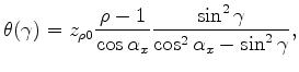
As shown in Biondi (2003) Chap 11, in the case of constant velocity error, the residual moveout of an ADCIG gather is
where
 and
and
Therefore we introduce the moveout parameter
The derivative is
Define
 |
|||
 |
 relation (see appendix B):
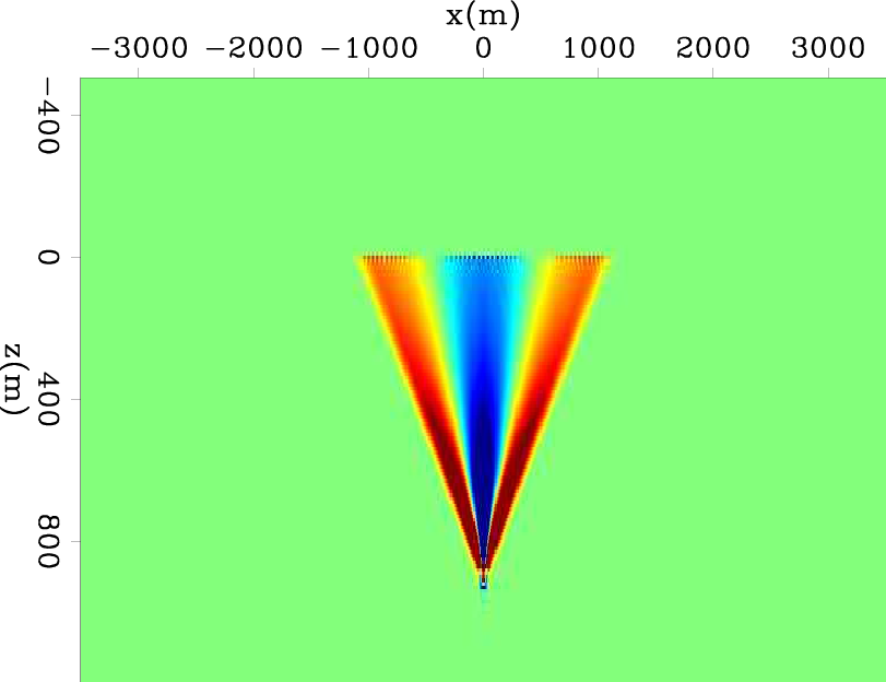
The sensitivity kernel
calculated using the direct operator and the indirect operator
are shown in figure 2, as with the Toldi operator (Toldi, 1985), the characteristic shape of
such a sensitivity kernel is a center lobe, with two side lobes with oppositite polarity, which reaffirms the well known fact
that velocity perturbation at the center and the side-end lateral position will change the curvature of ADCIGs towoard opposite directions.
Yet the overall average is positive, which would give the correct update in case of a bulk shift slowness error.

|
|---|
|
sensKer1w.bf2,sensKer1w.bf1m
Figure 2. Sensitivity kernel |
|
|
Now if we review this method on eq. (6), the success of this method simply relies on the proper behavior of
the two components in eq. (6):
![]() needs to correctly detect the curvature of the ADCIGs so that the inversion will choose a moveout direction that properly flatten the gathers;
needs to properly convert the curvature perturbation to the update in slowness space.
needs to correctly detect the curvature of the ADCIGs so that the inversion will choose a moveout direction that properly flatten the gathers;
needs to properly convert the curvature perturbation to the update in slowness space.
In cases where velocity error is big, the actual curvature of the gather may be poorly
represented the
![]() term. To further improve the robustness and precondition the gradient, the
analytic expression of
term. To further improve the robustness and precondition the gradient, the
analytic expression of
![]() in eq. (6) is replaced by a numerical approach. First a semblance
panel of
in eq. (6) is replaced by a numerical approach. First a semblance
panel of ![]() will be calculated. To ensure that the derivative at
will be calculated. To ensure that the derivative at ![]() can determine the correct curvature
that maximizes the semblance value, a Gaussian derivative rather than a simple
can determine the correct curvature
that maximizes the semblance value, a Gaussian derivative rather than a simple ![]() finite-difference derivative is applied. The width of the Gaussian can be reduced in later iterations.
finite-difference derivative is applied. The width of the Gaussian can be reduced in later iterations.
|
|
|
|
Moveout-based wave-equation migration velocity analysis |
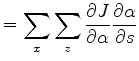
![$\displaystyle \frac{\partial J}{\partial s} \vert _{s=s_0} =
\sum_{x}\sum_{z} ...
...mma,z,x;s_0)g(\gamma)\frac{\partial{\alpha}}{\partial{s}}) \right]
\right\} .
$](img53.png)