|
|
|
|
Random boundary condition for low-frequency wave propagation |
|
|---|
|
srctwentyfive
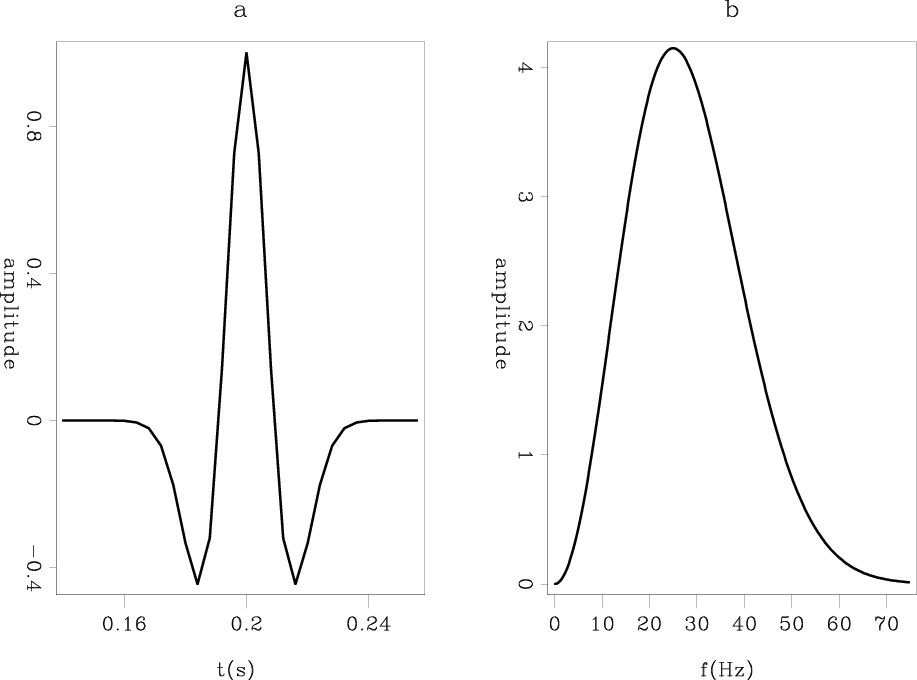
Figure 4. Time-domain and frequency-domain broadband source with a peak frequency of |
|
|

|
|---|
|
wvmvtwentyfivehoriz
Figure 5. Time domain wavefield snapshots for a broadband point source with a peak frequency of |
|
|
In this section, we test a broadband point source with a peak frequency of ![]() Hz, using the same boundary as in the previous example. Figure 4 shows the amplitude spectrum of the point source used, which contains non-trivial high- and low-frequency components. Figure 5 (top row) shows 2D slices of the wavefield using one realization of each velocity. In this case, the proposed random boundaries still work quite well. A random boundary with a small grain size is effective at high frequency, but has difficulty eliminating low-frequency components of the source. This is more obvious in the bottom row of Figure 5, which is the stacked wavefield of the same source and record time, using
Hz, using the same boundary as in the previous example. Figure 4 shows the amplitude spectrum of the point source used, which contains non-trivial high- and low-frequency components. Figure 5 (top row) shows 2D slices of the wavefield using one realization of each velocity. In this case, the proposed random boundaries still work quite well. A random boundary with a small grain size is effective at high frequency, but has difficulty eliminating low-frequency components of the source. This is more obvious in the bottom row of Figure 5, which is the stacked wavefield of the same source and record time, using ![]() different realizations of random boundaries.
different realizations of random boundaries.
|
|
|
|
Random boundary condition for low-frequency wave propagation |