|
|
|
|
Random boundary condition for low-frequency wave propagation |
|
|---|
|
velfullrndbnd
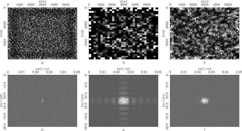
Figure 6. Velocity field with different random boundaries: a) cubic grains with |
|
|
Another way to analyze the previous two examples is to consider the spectra of different random boundaries. Figure 6 shows a velocity field filled with different random boundaries. We can look at their ![]() spectra by Fourier transform along both the
spectra by Fourier transform along both the ![]() and
and ![]() axes and take the absolute amplitudes (Figure 6). It can be seen that randomly shaped grains at high
axes and take the absolute amplitudes (Figure 6). It can be seen that randomly shaped grains at high ![]() values have an amplitude similar to that of single-cell random boundary, and at low
values have an amplitude similar to that of single-cell random boundary, and at low ![]() values have an amplitude similar to that of a large cubic-grain random boundary. The large cubic-grain random boundary, on the other hand, has a far lower high-
values have an amplitude similar to that of a large cubic-grain random boundary. The large cubic-grain random boundary, on the other hand, has a far lower high-![]() component, and there are even notches at certain
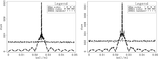
component, and there are even notches at certain ![]() values. These features become obvious in stacked
values. These features become obvious in stacked ![]() and
and ![]() spectra of each random field (Figure 7). Large amplitude at high
spectra of each random field (Figure 7). Large amplitude at high ![]() values means more detailed randomness, which is useful for scattering high-frequency waves. Large amplitude at low
values means more detailed randomness, which is useful for scattering high-frequency waves. Large amplitude at low ![]() values means many coarse ``grains'', which is useful for scattering low-frequency waves. Random fields that have both can effectively scatter broadband signals, and this is the case for randomly shaped grains. The large volume of the grains effectively scatters low-frequency signals, while the edges of grains effectively scatter high-frequency signals. On the other hand, regular notches in the spectrum mean that the random field (cubic grains in this case) displays certain patterns that will render it unable to deal with certain wavefronts; this is analogous to the null space in inversion.
values means many coarse ``grains'', which is useful for scattering low-frequency waves. Random fields that have both can effectively scatter broadband signals, and this is the case for randomly shaped grains. The large volume of the grains effectively scatters low-frequency signals, while the edges of grains effectively scatter high-frequency signals. On the other hand, regular notches in the spectrum mean that the random field (cubic grains in this case) displays certain patterns that will render it unable to deal with certain wavefronts; this is analogous to the null space in inversion.
|
|---|
|
vkabsstk
Figure 7. Stacked |
|
|
|
|
|
|
Random boundary condition for low-frequency wave propagation |