Ambient seismic noise eikonal tomography for near-surface imaging at Valhall

Scholte-wave velocity maps

Correlations were performed for time blocks of at most 3 hours. Signal to noise ratios were calculated using a moveout window 4 seconds wide centered on a moveout-velocity trajectory of 350 m/s. For the inversion we only used picks with SNR’s of over 2 that were located within a radius of 1750 m of the virtual-source gather. We found the eikonal tomography results to be more improved by excluding picks at larger offsets than by elevating the SNR threshold. Further offsets might get sensitive to deeper structures or contain other wavemodes. Thus the gradients would fundamentally start to conflict. Figures 7-9 contain images of Scholte-wave velocities and quality factors obtained by performing eikonal tomography on the 2004, 2005 and 2008 datasets, respectively. The top left panels show the expected-value velocity maps, and the top right panels show the associated standard deviations. 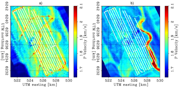The lower left and right panels show maps of the regularized pick density and the number of estimates ($N$ ), respectively. For comparison, Figure 10 shows maps of estimated P-wave (not Scholte-wave) velocities between 60 and 105 m (in Figure 10a) and between 150 and 195 m (in Figure 10b) beneath the ocean floor. This result was obtained by Sirgue et al. (2010) using full-waveform inversion (FWI) between 3.5 Hz and 7 Hz on a conventional active seismic dataset.

Several high- and low-velocity anomalies can be distinguished in the Scholte-wave maps from the 2004 and 2005 data. These appear to correspond to structures also observable in the P-wave velocity map. The high-velocity anomalies are interpreted to be channel features (indicated by arrows). Dotted circles indicate two distinct low-velocity zones. The FWI inversion was performed for frequencies higher than those in this eikonal tomography study, so it is not surprising that the tomographic images of Scholte-wave velocities obtained from the eikonal tomography lack the short-wavelength resolution of the P-wave velocity map obtained from FWI.

The traveltime map estimated from the 2008 dataset contains generally higher velocitiesthan the traveltime maps from the 2004 and 2005 datasets. This might be because the (unfiltered) 2008 dataset contains stronger low frequencies, and thus is more sensitive to higher velocities deeper in the Earth. However, parts of the 2008 map (especially in the South) bear little resemblance to the 2004 or 2005 maps, or to the structures in the P-wave velocity map. Only 2 hours of data were available from 2008, and as a result the SNR’s of the virtual-source gathers generally were lower. The 2008 Scholte-wave velocity map was thus constructed using far fewer accepted picks than the maps of 2004 and 2005, so the map from the 2008 dataset may simply be unreliable. Availability of longer data sets recorded without a low-cut filter would enable further investigation of the application of the lower frequencies in the microseism energy to subsurface imaging.

Note the isolated low near the center of the array in the pick-density map for the 2004 eikonal inversion. This receiver station was probably malfunctioning (or possibly was simply mislocated) and slipped through initial quality control. It did not damage the results, however, because it was discarded by the automated picking algorithm. The P-wave velocity map in Figure 10b prominently displays a large meandering channel that passes under the extreme southeastern part of the array. This channel is deeper than the narrower channels marked by the meandering dotted arrows in Figure 10b. There is no corresponding anomaly in the eikonal result for the 2004 data. There are anomalies in the 2005 and 2008 data at approximately the right location, but they are certainly not conclusive matches. It is possible that the lower-frequency, deeper-sensing 2008 dataset might be detecting that channel. Unfortunately the edges of the array have relatively few travel times to work with, so this remains inconclusive. Note that FWI was able to use active sources, which covered a wider area, to image well outside the receiver array even at these shallow depths. Interferometry uses the receivers as sources and so has a more restricted image space.

Artman-V-Etom
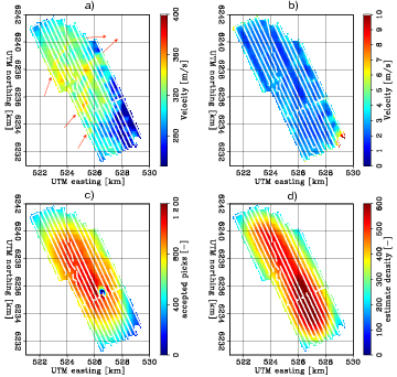
Figure 7. Images of Scholte-wave velocities and uncertainties obtained from eikonal tomography on the 2004 dataset; the expected value (a), the standard deviation of velocity (b), pick density at each station (c), and the number of velocity estimates at each grid point (d). Dotted arrows in (a) indicate channel features.

Jianhua-V-Etom
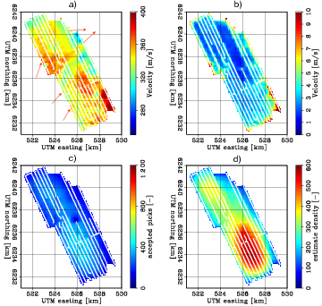
Figure 8. Images of Scholte-wave velocities and uncertainties obtained from eikonal tomography on the 2005 dataset; the expected value (a), the standard deviation of velocity (b), pick density at each station (c), and the number of velocity estimates at each grid point (d). Dotted arrows in (a) indicate channel features.

Laura-V-Etom
Figure 9. Images of Scholte-wave velocities and uncertainties obtained from eikonal tomography on the 2008 dataset; the expected value (a), the standard deviation of velocity (b), pick density at each station (c), and the number of velocity estimates at each grid point (d). Dotted arrows in (a) indicate channel features. This dataset produces a distinctly different result from the other two, possibly because it was recorded without a low-cut recording filter.

Valhall-Laurent-FWI
Figure 10. Images of average P-wave velocities obtained using waveform inversion (Sirgue et al., 2010) of active P-wave data; (a) between 60 and 105 m beneath the ocean floor, and (b) between 150 and 195 m beneath the ocean floor. Dotted arrows indicate channel features; dotted circles indicate two distinct low-velocity zones.

Ambient seismic noise eikonal tomography for near-surface imaging at Valhall