|
|
|
|
Ambient seismic noise eikonal tomography for near-surface imaging at Valhall |
 virtual-source gathers, one at each receiver station, and applying the acceptence criteria mentioned above leads to a set of estimates of the local wave velocity at each receiver location
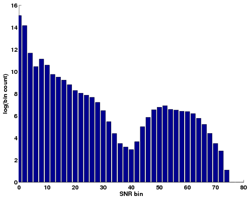
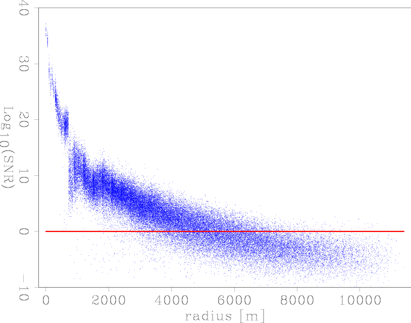
A logarthmic histogram of the SNR of all picks in the Valhall array (Figure 4(a)) shows the large majority of picks have very low SNR. Generally the SNR ratio decreases quite rapidly with increasing source-receiver distance due to geometrical spreading (Figure 4(b)). The deficiency between SNR's of 30 to 40 and the jump in the SNR scatter plots at a radius of ![]() m are related to the dispersion of the Scholte wave in the correlation gathers. They coincide with phase cycles, which are strongly reflected in the amplitude of the envelope function.
m are related to the dispersion of the Scholte wave in the correlation gathers. They coincide with phase cycles, which are strongly reflected in the amplitude of the envelope function.
|
|---|
|
snrhist,snrscat
Figure 4. a) Histogram of SNR. b) Scatter plot of 1% of all SNR's versus radius, line is the lower acceptence level. |
|
|
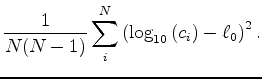
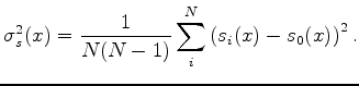
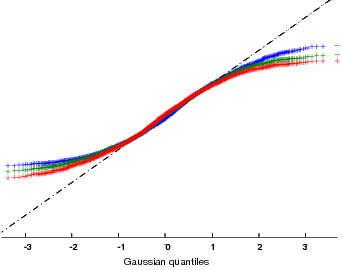
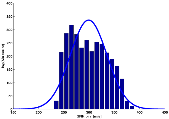
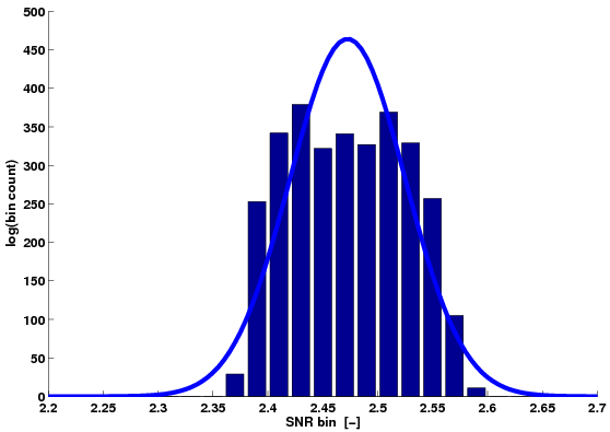
A complication with Gaussian statistics on measurements of velocity or slowness is that they are both always positive. Tarantola (2006) suggests these so called Jeffreys quantities are more safely analyzed in their logarithmic magnitudes. Here we briely disuss the model estimate distributions. The expected value and variance of the estimate sets are calculated on the estimates in three magnitudes: linear slowness, linear velocity and logarithm of velocity. For linear slowness magnitudes we have (again)
| (4) |
 |
(5) |
| (6) |
 |
(7) |
 |
(8) |
 |
|||
 |
(9) |
The results of either approach are most intuitively compared in units of velocity (m/s). So the expected values are compared through:
Normal distributions are fitted to the estimates in Figures 5 and 6 on the respective magnitudes.
For the estimates near a high-velocity anomaly we find 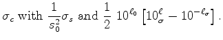 m/s and
![]() m/s,
m/s,
![]() m/s and
m/s and
![]() m/s, and
m/s, and
![]() m/s and
m/s and
![]() m/s.
For the estimates near a low-velocity anomaly we find
m/s.
For the estimates near a low-velocity anomaly we find ![]() m/s and
m/s and
![]() m/s,
m/s,
![]() m/s and
m/s and
![]() m/s, and
m/s, and
![]() m/s and
m/s and
![]() m/s.
For both estimate sets we find the expected value on the logarithmic velocity magnitude to be within the values of the expected value on the linear slowness and linear velocity magnitudes.
However the deviations on these expected values are about 10 times smaller then the standard deviations on the estimates, regardless of which magnitudes are analyzed.
m/s.
For both estimate sets we find the expected value on the logarithmic velocity magnitude to be within the values of the expected value on the linear slowness and linear velocity magnitudes.
However the deviations on these expected values are about 10 times smaller then the standard deviations on the estimates, regardless of which magnitudes are analyzed.
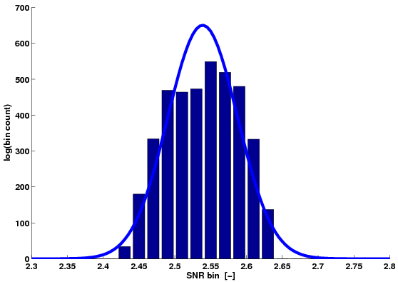
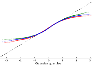
In Figures 5(d) and 6(d) Q-Q plots indicate how well the estimates fit normal distributions (plus symbols for slowness magnitudes, circles for velocity magnitudes and quandrangles for logarithmic velocity magnitudes). Q-Q plots for the different magnitudes carry a different unit on their vertical axis. The diagonal corresponds to a perfect fit. The intermediate quantiles follow Gaussian statistics quite well. In the lower and higher quantiles the data differs from a normal distribution. In the high-velocity anomaly (Figure 5(d)) the slowness magnitudes fit a normal distribution better in the lower quantiles and the velocity magnitudes better in the higher quantiles (not surprising because velocity is inverse slowness). In the low-velocity anomaly (Figure 6(d)) the logarithmic velocity magnitudes fit a normal distribution best in the lower quantiles while the velocity magnitudes better in the higher quantiles.


|
|---|
|
estimates1a,estimates1b,estimates1d,fits1
Figure 5. Histograms and their normal distribution fits of the gradient estimates in a high velocity region: a) linear slowness magnitude, b) linear velocity magnitude, c) logarithmic velocity magnitude, d) normal Q-Q plots of the gradient magnitudes (plus symbols: linear slowness, circles: linear velocity, quandrangles: logarithmic velocity). |
|
|
|
|---|
|
estimates2a,estimates2b,estimates2d,fits2
Figure 6. Histograms and their normal distribution fits of the gradient estimates in a low-velocity region: a) linear slowness magnitude, b) linear velocity magnitude, c) logarithmic velocity magnitude, d) normal Q-Q plots of the gradient magnitudes (plus symbols: linear slowness, circles: linear velocity, quandrangles: logarithmic velocity). |
|
|
These observations might not hold in general for low- and high-velocity anomalies. Fortunately, the choice of which magnitude to use to analyze the gradient estimates does not significantly change the resulting tomography maps.
Gaussian statistics do not adequately fit the tails of the estimate sets.
For simplicity we chose to base the tomographic images on the expected value
of a linear slowness basis.
For this data, the variance is a very limited measure and does not infer an estimate certainty in a Gaussian statistics sense.
Thus two additional quality measures of the expected value are the density of accepted picks and the
velocity-estimate density. The first is a (regularized) map of the number of accepted travel time
picks per station. The second is simply a map of
, the number of raw travel time measurements
available at that location.
|
|
|
|
Ambient seismic noise eikonal tomography for near-surface imaging at Valhall |