An approximation of the inverse Ricker wavelet as an initial guess for bidirectional deconvolution

Synthetic data example

First we test our initial guess on synthetic data. Because we hope to improve the deconvolution of data with a Ricker-like wavelet, we will test the synthetic data with a Ricker wavelet. We use a 2D reflectivity model to generate our synthetic data. Figure 8(a) shows the model we used, and Figure 1(a) shows our approximate Ricker wavelet (fourth-order) that we used to generate our data. The final synthetic data is shown in Figure 9(a). The wavelet we used is causal, hence we have some time lag in our synthetic data then the spiky model. We use the same deconvolution filter for all traces in our synthetic data example. Figures 10(a) and 10(b) are the result of bidirectional deconvolution using a spike as initial filters for $f_a$ and $f_b^r$ . Figures 11(a) and 11(b) are the result of deconvolution using our approximate inverse Ricker wavelet with $\rho$ =0.7. We see both of the initial guesses (the simple spike and our inverse Ricker wavelet) did a reasonably good job if we see the global view. If we examine the result carefully, we find that the result with the inverse Ricker wavelets as initial guesses has less ghosting, especially in the vicinity of 1.0 s to 1.2 s and 3 km to 5.4 km. This may be more obvious if we see the magnified views of the results. We can also compare them to the magnified views of the synthetic data (Figure 9(b)) and the model (Figure 8(b)), and we find both of bidirectional deconvolution results improve the resolution of events. Figures 12(a) and 12(b) are magnified wiggle plots in the same time window but for just a single trace in the vicinity of 4000 m of CMP_x, from which we can see the the result with inverse Ricker initial guess has less ghosting in wiggle. Although there is improvement, it is not very significant for our synthetic case.

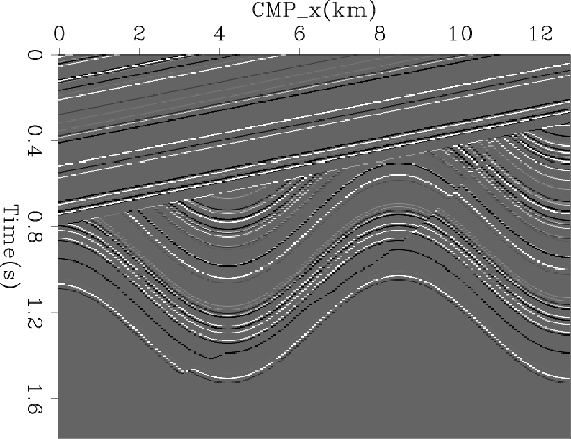
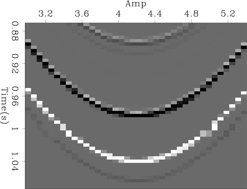
2d-synthetic-model,2d-synthetic-model-local
Figure 8. 2D reflection model we used to to generate our synthetic data: (a) the global view; (b) the magnified view in the time window from .872 s to 1.072 s and in CMP_x range from 3 km to 5.4 km.

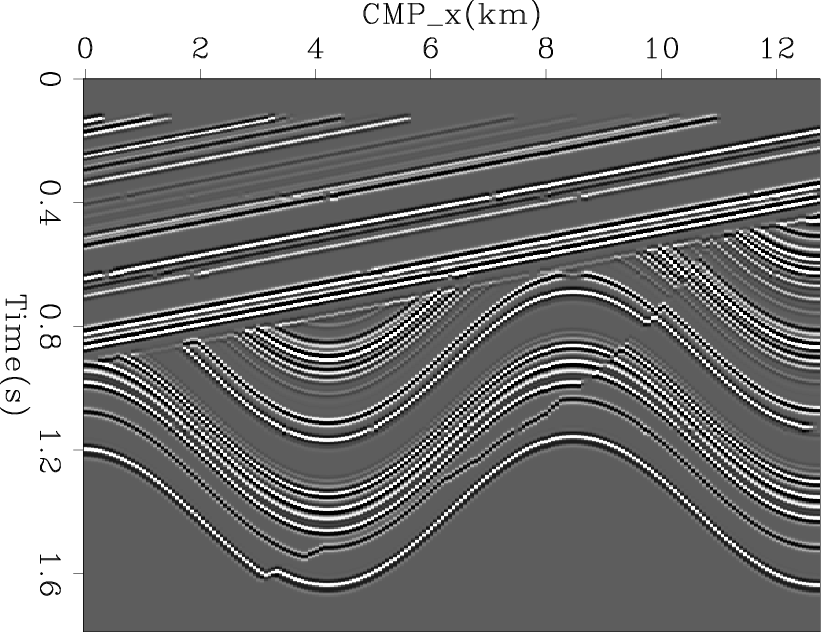
2d-synthetic-data,2d-synthetic-data-local
Figure 9. The synthetic data we used for our test: (a) the global view; (b) the magnified view in the time window from 1 s to 1.2 s and in CMP_x range 3 km to 5.4 km.

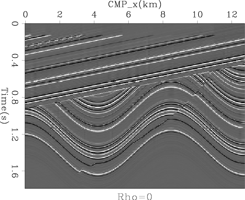
result-rho-0,result-local-rho-0
Figure 10. The result of bidirectional deconvolution using a spike as initial filters $f_a$ and $f_b^r$ on synthetic data: (a) the global view; (b) the magnified view in the time window from 1 s to 1.2 s and in CMP_x range 3 km to 5.4 km.

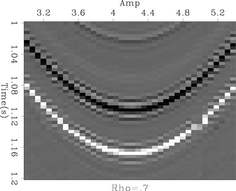
result-rho-7,result-local-rho-7
Figure 11. The result of bidirectional deconvolution using our approximate inverse Ricker wavelet with $\rho$ =0.7 on synthetic data: (a) the global view; (b) the magnified view in the time window from 1 s to 1.2 s and in CMP_x range 3 km to 5.4 km.

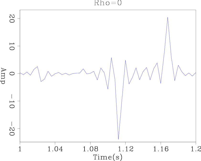
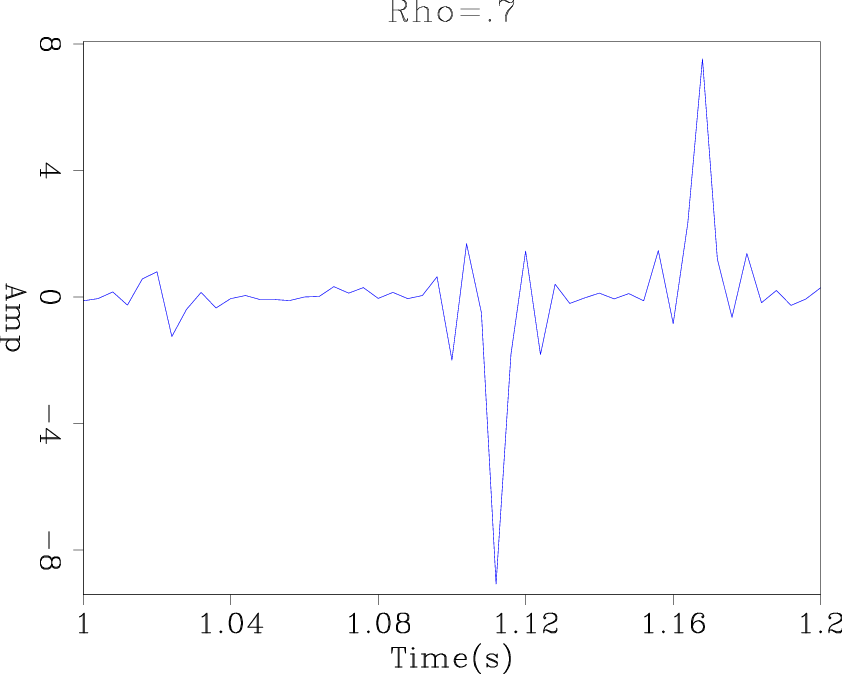
wiggle-local-rho-0,wiggle-local-rho-7
Figure 12. The magnified wiggle plot of the bidirectional deconvolution results at cmp=4.3 km in the time window from 1 s to 1.2 s: (a) with a spike as the initial guess; (b) with an inverse Ricker wavelet as the initial guess.

An approximation of the inverse Ricker wavelet as an initial guess for bidirectional deconvolution