An approximation of the inverse Ricker wavelet as an initial guess for bidirectional deconvolution

Field data example

We also test our initial guess on a marine common-offset 2D data set. We use the same deconvolution filter for all traces in our field data example as well. Figure 13 shows the 2D input data set. Figure 14 shows the bidirectional deconvolution result with a simple spike as the initial guesses and Figure 15 shows the bidirectional convolution with our inverse Ricker wavelet as the initial guesses, using $\rho$ =0.8.

2d-field-data
Figure 13. A marine common-offset 2D data set we used for our test.

result-0
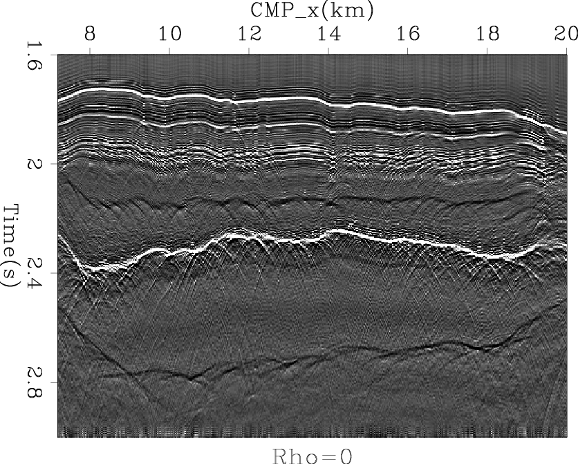
Figure 14. The result of deconvolution using a spike as initial filters $f_a$ and $f_b^r$ on field data.

result-8
Figure 15. The result of deconvolution using our approximate inverse Ricker wavelet with $\rho$ =0.8 on field data.

It is obvious that the result of using the inverse Ricker wavelet as an initial guess is much better. For example, the ghost events before the first reflection are much suppressed, and the upper boundary of the salt body, which is the event from about 2.2 s to 2.4 s, is condensed. There appears to be a polarity change plus a time shift in our two bidirectional deconvolution output results with different initial guesses. This is not an error. Given the wavelets estimated from deconvolution process, it is a reasonable result.

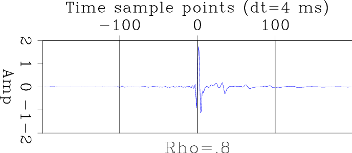
Figures 16(a) and 16(b) are the wavelets estimated by a simple spike initial guess and our inverse Ricker wavelet initial guess with $\rho$ =0.8. On these wavelet, we can clearly see the airgun bubbles. And the time interval between bubbles are corelate the data shown in 13 very well. The wavelets are causal-like, or in other words, we do not have too much energy in the negative time before the first major impulse. These two evidence indicate that we estimate the wavelet of our field data correctly.However, we still have some problem here. We must mention that we tried to enlarge the filter length to get a longer estimated wavelet by the same scheme, but we got a noisy result. It seems we have some instability here, but we do not know the reason of this now. We are researching this and will explain the reason in furtrue report after we figure it out.

wavelet-0,wavelet-8
Figure 16. Estimated wavelet from bidirectional deconvolution on field data: (a) using a spike as initial filters $f_a$ and $f_b^r$ ; (b) using our approximate inverse Ricker wavelet with $\rho$ =0.8.

The two wavelets in Figures 16(a) and 16(b) look very similar, but have opposite polarity and a different origin in the time axis. The flipped polarity is caused by the origin shift. Since we have the same input data and wavelet for deconvolution, even with different initial guesses, we should get the same (or at least similar) estimated wavelet and deconvolution filter after the process. Bidirectional deconvolution forces the polarity of both the estimated wavelet and the deconvolution filter to be positive at the origin of the time axis. So if the origin of the estimated wavelet has been shifted from positive to negative, the polarity will be flipped. This estimated wavelet origin shift will cause the output of the deconvolution result to shift on the time axis as well.

An approximation of the inverse Ricker wavelet as an initial guess for bidirectional deconvolution