Reverse-time migration using wavefield decomposition

Wavefield decomposition

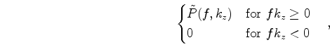
The conventional method for wavefield decomposition operates in the Fourier domain. This method was first applied to vertical seismic profiles (Hu and McMechan, 1987). Here, wavefields are decomposed into their upgoing and downgoing components in the F-K domain by using a 2-D fast Fourier transform (FFT):

$$\tilde{P}_{z+}(f,k_z) = \begin{cases} \tilde{P}(f,k_z) & \mbox{for }fk_z \ge 0 \\ 0 & \mbox{for }fk_z < 0 \end{cases} \quad ,$$ (11)

$$\tilde{P}_{z-}(f,k_z) = \begin{cases} 0 & \mbox{for }fk_z \ge 0 \\ \tilde{P}(f,k_z) & \mbox{for }fk_z < 0 \end{cases} \quad ,$$ (12)

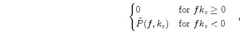where $\tilde{P}(f,k_z)$ is the 2-D Fourier transform of the wavefield $P(t,z)$ at any horizontal position $x$ , and $f$ and $k_z$ are the frequency and vertical wavenumber representations of the wavefield. Note that the wavefield $P(t,z)$ can be either the source wavefield $S(t,z)$ or the receiver wavefield $R(t,z)$ .

A similar method can be used to obtain the leftgoing and rightgoing components of wavefields:

$$\tilde{P}_{x+}(f,k_x) = \begin{cases} \tilde{P}(f,k_x) & \mbox{for }fk_x \ge 0 \\ 0 & \mbox{for }fk_x < 0 \end{cases} \quad ,$$ (13)

$$\tilde{P}_{x-}(f,k_x) = \begin{cases} 0 & \mbox{for }fk_x \ge 0 \\ \tilde{P}(f,k_x) & \mbox{for }fk_x < 0 \end{cases} \quad ,$$ (14)

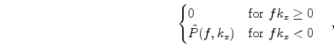where $\tilde{P}(f,k_x)$ is the 2-D Fourier transform of the wavefield $P(t,x)$ at any depth $z$ , and $f$ and $k_x$ are the frequency and horizontal wavenumber representations of the wavefield.

In this paper, I apply smooth-cut F-K filters to the wavefield decomposition instead of using the sharp-cut filters shown in Equations 3 to 6, so that noise due to the FFT of discontinuous functions is reduced. Using smooth-cut filters might slightly reduce the illumination of reflectivity images, but it is worth attentuating the noise from FFT.

The decomposed wavefields, as in Equations 3 to 6, are the the 2-D inverse Fourier transforms of the decomposed wavefields derived from Equations 11 to 14. Thus, the terms on the right-hand sides of Equations 3 to 6 are all complex. However, in each equation, the summation of the imaginary parts becomes zero, and the wavefield is equal to the summation of the real parts of the decomposed wavefields; for example,

$$S(t,\vec{x}) = S_{z+}(t,\vec{x}) + S_{z-}(t,\vec{x}),$$ (15)

$$= [ S_{z+}(t,\vec{x}) ] + [ S_{z-}(t,\vec{x}) ].$$ (16)

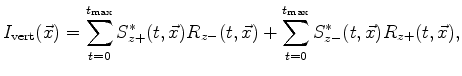
In their proposed imaging condition, Liu et al. (2007) applied only the real parts of the decomposed source and receiver wavefields to the imaging conditions in Equations 8 and 9. Thus, a question is raised about the effect that the imaginary components might have on the decomposed RTM images. Considering decomposed wavefields as complex functions, I rewrite Equations 8 and 9 to be

$$I_{\text{vert}}(\vec{x}) = \sum_{t=0}^{t_{\text{max}}} S^*_{z+}(t... ...t,\vec{x}) + \sum_{t=0}^{t_{\text{max}}} S^*_{z-}(t,\vec{x}) R_{z+}(t,\vec{x}),$$ (17)

and

$$I_{\text{horiz}}(\vec{x}) = \sum_{t=0}^{t_{\text{max}}} S^*_{x+}(... ...t,\vec{x}) + \sum_{t=0}^{t_{\text{max}}} S^*_{x-}(t,\vec{x}) R_{x+}(t,\vec{x}),$$ (18)

where an asterisk denotes the complex conjugate. Equations 17 and 18 can be computed using only the wavefield decomposition in the T-K domain (Liu et al., 2011). Thus, this method is practical, because there is no need to save wavefields at every time step.

Reverse-time migration using wavefield decomposition