 |
 |
 |
 | Wave-equation inversion of time-lapse seismic data sets |  |
![[pdf]](icons/pdf.png) |
Next: Example
Up: Ayeni and Biondi: 4D
Previous: Introduction
Given a linearized modeling operator  , the seismic data
  for survey
  due to a reflectivity model
  is
is
 |
(A-1) |
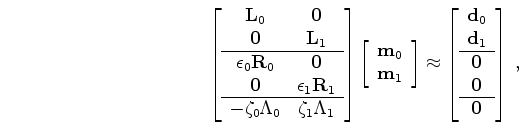
Assuming we have two data sets (baseline
 and monitor
 ) acquired at different times over an evolving reservoir, joint least-squares migration/inversion involves solving the regression
![\begin{displaymath}\begin{array}{ccc} \left [ \begin{array}{cc} {\bf L}_{0} & {\...
...0} \\ {\bf0} \\ \hline {\bf0} \end{array} \right ] \end{array},\end{displaymath}](img13.png) |
(A-2) |
where
 and
and
 are the spatial and temporal regularization operators respectively, and
 and
and
 are the corresponding regularization parameters.
Although we can directly solve equation 2 by minimizing the quadratic-norm of the regression (Ajo-Franklin et al., 2005), we choose to transform it to an image space problem of the form (Appendix A)
are the corresponding regularization parameters.
Although we can directly solve equation 2 by minimizing the quadratic-norm of the regression (Ajo-Franklin et al., 2005), we choose to transform it to an image space problem of the form (Appendix A)
![\begin{displaymath}\begin{array}{c} \left [ \begin{array}{ccc} {\bf H_0 } & {\bf...
...\\ \hline {\bf0} \\ {\bf0} \\ \end{array} \right ], \end{array}\end{displaymath}](img18.png) |
(A-3) |
where
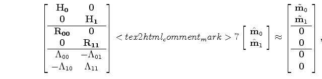 is the wave-equation Hessian, and
 and
and
 are the spatial and temporal constraints.
Note that
are the spatial and temporal constraints.
Note that
 , the migration operator, is the adjoint of the modeling operator
.
The inverted time-lapse image
, the migration operator, is the adjoint of the modeling operator
.
The inverted time-lapse image
 is then the difference between the inverted baseline and monitor images (
 and
and
 ).
Alternatively, we can re-write equation 3 to invert directly for the time-lapse image and a static baseline image (Appendix A).
Furthermore, equation 3 can be extended to multiple seismic data sets (Ayeni and Biondi, 2010).
).
Alternatively, we can re-write equation 3 to invert directly for the time-lapse image and a static baseline image (Appendix A).
Furthermore, equation 3 can be extended to multiple seismic data sets (Ayeni and Biondi, 2010).
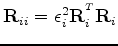
As shown in Appendix A, if there are physical movements of reflectors and velocity changes (e.g., due to reservoir depletion and compaction) between surveys, the baseline and monitor images will not be aligned.
Such misalignments must be accounted for before or during inversion.
As is the case in many practical time-lapse monitoring problems, we assume that the monitor data are migrated with the baseline velocity.
The updated inversion problem is then given by (Appendix A)
![\begin{displaymath}\begin{array}{c} \left [ \begin{array}{ccc} {\bf H }_{0} & {\...
...\\ \hline {\bf0} \\ {\bf0} \\ \end{array} \right ], \end{array}\end{displaymath}](img26.png) |
(A-4) |
where
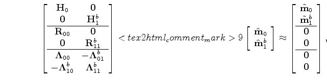 and
and
 are respectively the migrated and inverted monitor images repositioned (warped) to the baseline image.
The superscript
are respectively the migrated and inverted monitor images repositioned (warped) to the baseline image.
The superscript  on the operators denotes that they are referenced to the baseline image.
For example,
on the operators denotes that they are referenced to the baseline image.
For example,
 is the Hessian matrix with the monitor geometry but with the baseline velocity.
Note that whereas the conventional time-lapse image
is the Hessian matrix with the monitor geometry but with the baseline velocity.
Note that whereas the conventional time-lapse image
 estimated at the baseline position is given by
 |
(A-5) |
the inverted time-lapse image
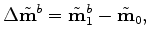 is given by
 |
(A-6) |
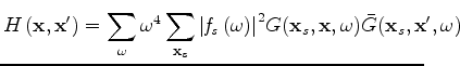
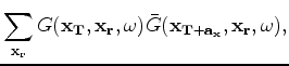
The wave-equation Hessian at image point 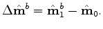 is defined as (Valenciano et al., 2006; Plessix and Mulder, 2004)
 |
|
|
|
 |
|
|
(A-7) |
where 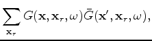 denotes all image points,
  is the complex conjugate of Green's function
  at frequency
  ,
,
 is the source function, and
 and
and
 are the source and receiver positions, respectively.
For any practical application, it is infeasible (and unnecessary) to compute the full Hessian matrix.
Because the problem is posed in the image space, we only need to compute the Hessian for a target region of interest around the reservoir.
In addition, we only compute off-diagonal elements sufficient to capture the dominant structure of the Hessian.
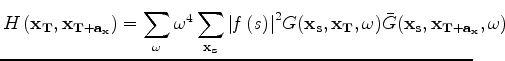
This target-oriented approximation of the Hessian is given by (Valenciano et al., 2006)
are the source and receiver positions, respectively.
For any practical application, it is infeasible (and unnecessary) to compute the full Hessian matrix.
Because the problem is posed in the image space, we only need to compute the Hessian for a target region of interest around the reservoir.
In addition, we only compute off-diagonal elements sufficient to capture the dominant structure of the Hessian.
This target-oriented approximation of the Hessian is given by (Valenciano et al., 2006)
 |
|
|
|
 |
|
|
(A-8) |
where
 is an image point within the target area, and
 represents points within a small region around
.
For any image point, elements of
represents points within a small region around
.
For any image point, elements of
 represents a row of a sparse Hessian matrix
 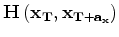 whose non-zero components are defined by
 .
Therefore,
defines the how many off-diagonal elements of the Hessian are computed -- which represents the size of the point spread function (PSF) around each image point.
Note that because of symmetry, only one half of the approximate Hessian is required.
The target-oriented Hessian and computational savings are discussed in further detail by Valenciano et al. (2006) and Tang (2008).
.
Therefore,
defines the how many off-diagonal elements of the Hessian are computed -- which represents the size of the point spread function (PSF) around each image point.
Note that because of symmetry, only one half of the approximate Hessian is required.
The target-oriented Hessian and computational savings are discussed in further detail by Valenciano et al. (2006) and Tang (2008).
In this paper, the spatial regularization operators are non-stationary dip filters.
First, we estimate the local dips on the migrated baseline image using a plane-wave destruction method (Fomel, 2002).
Then we construct the operator based on factorization of directional Laplacian representations of the local dip filters (Hale, 2007).
The temporal constraint is implemented as a difference between the aligned images.
To attenuate multiples and other unwanted artifacts in the data, we perform a high-resolution Radon demultiple on the data.
In order to align the baseline and monitor images prior to inversion, we perform pre-stack warping using a cyclic local cross-correlation method (Ayeni, 2010).
In the next section, we apply the proposed method to a field time-lapse data set.
We show applications to complete and incomplete monitor data sets.
|
|
|
|
| Wave-equation inversion of time-lapse seismic data sets | |
|
Next: Example
Up: Ayeni and Biondi: 4D
Previous: Introduction
2011-05-24