|
|
|
|
Migration velocity analysis for anisotropic models |
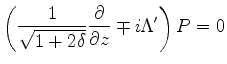
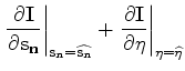
Anisotropic MVA is a non-linear inversion process that aims to find
the background anisotropic model that minimizes the residual image
![]() . The residual image is derived
from the background image
. The residual image is derived
from the background image ![]() , which is computed with the current
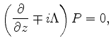
background model. To form the image, both the source and receiver
wavefields are downward continued using the one-way wave equations. Assuming that the shear velocity is much
smaller than the P-wave velocity, one way of formulating up-going and
down-going one-way acoustic wave equations for VTI is shown as follows
(Shan, 2009):
, which is computed with the current
background model. To form the image, both the source and receiver
wavefields are downward continued using the one-way wave equations. Assuming that the shear velocity is much
smaller than the P-wave velocity, one way of formulating up-going and
down-going one-way acoustic wave equations for VTI is shown as follows
(Shan, 2009):
 is the wavefield in the space-frequency
domain and
is the wavefield in the space-frequency
domain and  is the spatial wavenumber vector.
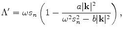
Many authors (Alkhalifah and Tsvankin, 1995; Tsvankin and Thomsen, 1994) have shown that P-wave
traveltime can be characterized by the NMO slowness, ![]() , and the
anellipticity parameter
, and the
anellipticity parameter ![]() . Therefore, the one-way wave-equation
in terms of
. Therefore, the one-way wave-equation
in terms of ![]() ,
, ![]() and
and ![]() is:
is:
 , are
coupled with each other. This is a theoretical proof of the well-accepted
observation that
, are
coupled with each other. This is a theoretical proof of the well-accepted
observation that
Notice that when  , the dispersion relationship ( equation
4) is the
same as the isotropic dispersion relationship, and the corresponding
one-way wave equation ( equation 6) is almost the
same as for the isotropic case, except for a depth stretch caused by
, the dispersion relationship ( equation
4) is the
same as the isotropic dispersion relationship, and the corresponding
one-way wave equation ( equation 6) is almost the
same as for the isotropic case, except for a depth stretch caused by
![]() . In other words, an elliptic anisotropic wavefield inversion is almost
equivalent to an isotropic wavefield inversion. Plessix and Rynja (2010)
reached the same conclusions for full-waveform inversion
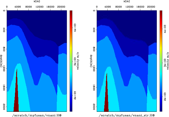
(FWI). Figure 1 compares the original
NMO velocity to the stretched NMO velocity. Notice that the geological
features are stretched downward for positive
. In other words, an elliptic anisotropic wavefield inversion is almost
equivalent to an isotropic wavefield inversion. Plessix and Rynja (2010)
reached the same conclusions for full-waveform inversion
(FWI). Figure 1 compares the original
NMO velocity to the stretched NMO velocity. Notice that the geological
features are stretched downward for positive ![]() . Because we
ignore
. Because we
ignore ![]() in the inversion, we expect the inverted NMO velocity
to have more similarity to the stretched NMO velocity than to the original one.
in the inversion, we expect the inverted NMO velocity
to have more similarity to the stretched NMO velocity than to the original one.
|
|---|
|
nmo
Figure 1. (a) Original NMO velocity for the anisotropic Hess model; (b) Stretched NMO velocity according to |
|
|
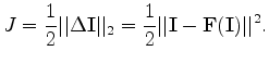
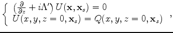
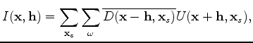
In general, the residual image is defined as (Biondi, 2008)
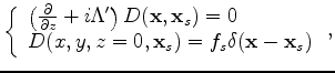
To perform MVA for anisotropic parameters, we first need to extend the
tomographic operator from the isotropic medium (Shen, 2004; Sava, 2004; Guerra et al., 2009) to the anisotropic medium. We define the
wave-equation tomographic operator T for anisotropic models as
follows:
 and anellipticity parameter
 | (10) |
 is the source wavefield at the image
point
is the source wavefield at the image
point
The dispersion relationship in equation (4) can be approximated with a rational function by Taylor series and Padé expansion analysis (Shan, 2009):
 . Equation (13) using binomial expansion can be further expanded to polynomials:
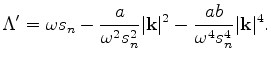 with respect to
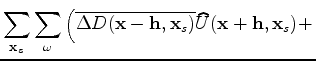
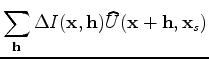
The background image is computed by applying the cross-correlation imaging condition:
 is the subsurface half-offset.
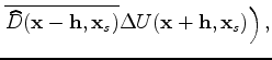
Perturbing the wavefields in equation (15) and ignoring the higher-order term, we can get the perturbed image as follows:
is the subsurface half-offset.
Perturbing the wavefields in equation (15) and ignoring the higher-order term, we can get the perturbed image as follows:
 and
and
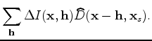
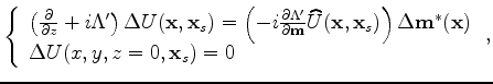
To evaluate the adjoint tomographic operator
![]() , which
maps from the image perturbation to the model perturbation, we first
compute the wavefield perturbation from the image perturbation using
the adjoint imaging condition:
, which
maps from the image perturbation to the model perturbation, we first
compute the wavefield perturbation from the image perturbation using
the adjoint imaging condition:
 is the row vector
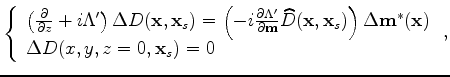
During the inversion, the model perturbation is unknown, and in fact must be estimated. Therefore, we obtain the image perturbation by applying a focusing operator (equation 7) to the current background image. Then the perturbed image is convolved with the background wavefields to get the perturbed wavefields (equation 17). The scattered wavefields are obtained by applying the adjoint of the one-way wave-equations (18) and (19). Finally, the model-space gradient is obtained by cross-correlating the upward propagated scattered wavefields with the modified background wavefields [the terms in the parentheses on the right-hand sides of equations (18) and (19)].
|
|
|
|
Migration velocity analysis for anisotropic models |