|
|
|
|
Imaging using compressive sensing |
Sub-surface offset gathers potentially represent an even higher, up to six, dimensional
problem. To test compressibility, I used a 4-D volume (![]() ) of dimensions (32,32,400,64).
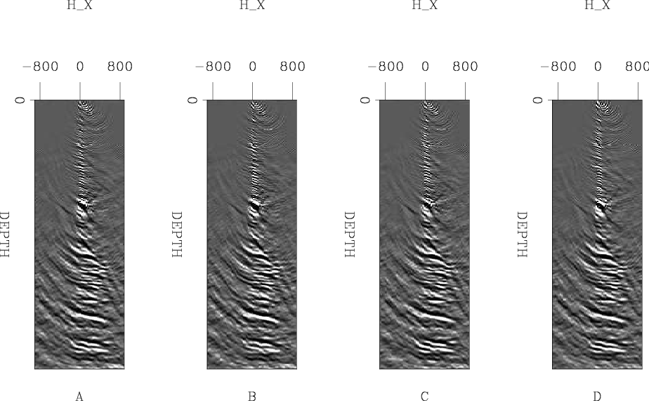
Figure 2 shows one of these sub-surface offset gathers and its neighbors, note
the similarly. Following Villasenor et al. (1996), I chose the 9/7 bi-orthonormal
transform(Antonini et al., 1992) used in JPEG compression.
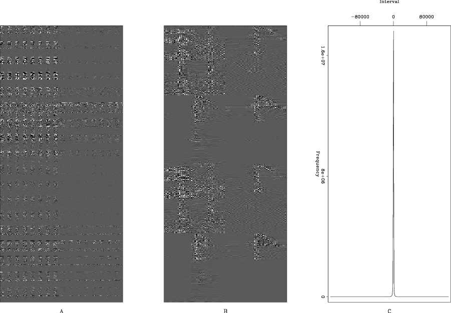
Figure 3 shows the resulting transform space and a histogram
of the absolute values. I then used several different
thresholds (throwing away 90%, 95%, 98%, and 99% of the data in the wavelet domain).
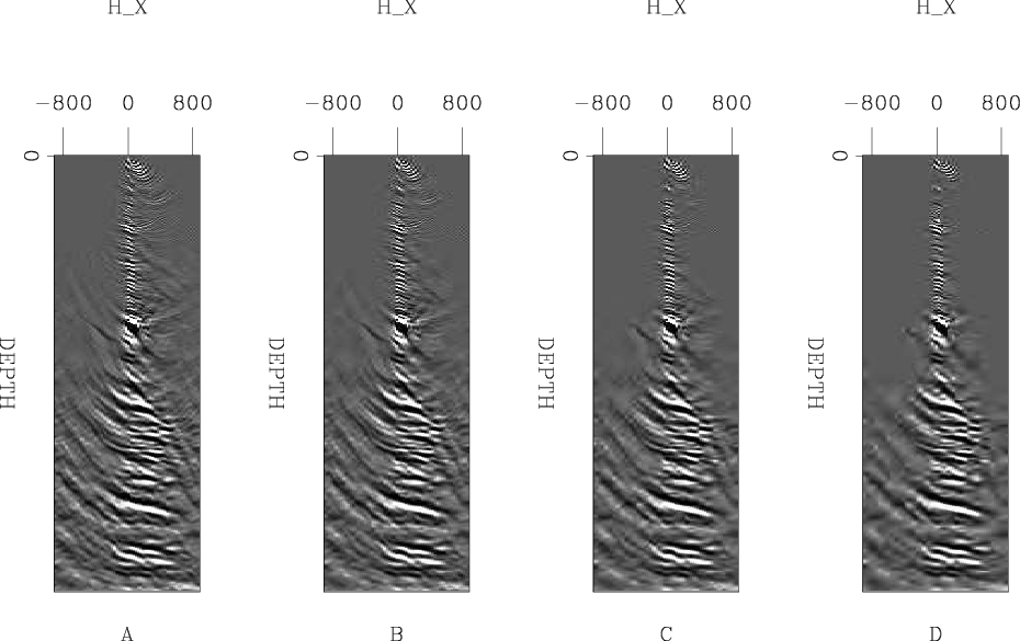
Figure 4
shows the result of transforming this thresholding volume back into the space-domain.
The resulting images are near-perfect at 95% and potentially acceptable at 98%. This translates
into an acceptable compression ratio of approximately 30:1.
) of dimensions (32,32,400,64).
Figure 2 shows one of these sub-surface offset gathers and its neighbors, note
the similarly. Following Villasenor et al. (1996), I chose the 9/7 bi-orthonormal
transform(Antonini et al., 1992) used in JPEG compression.
Figure 3 shows the resulting transform space and a histogram
of the absolute values. I then used several different
thresholds (throwing away 90%, 95%, 98%, and 99% of the data in the wavelet domain).
Figure 4
shows the result of transforming this thresholding volume back into the space-domain.
The resulting images are near-perfect at 95% and potentially acceptable at 98%. This translates
into an acceptable compression ratio of approximately 30:1.
|
|---|
|
raw
Figure 2. Five sub-surface offset gathers. B and C are one midpoint in X before and after A. E is one midpoint in Y before A. Note the spatial similarity, which lends itself to compression. |
|
|
|
|---|
|
wavelet1
Figure 3. Panel A shows the wavelet domain representation of the 4-D volume used in this experiment. Panel B shows a zoom into portion of the wavelet domain. Panel C shows a histogram of the wavelet domain values. Note how the vast majority of the values are nearly zero. |
|
|
|
|---|
|
offset
Figure 4. The result of zeroing the smallest values of the wavelet domain representation shown in Figure 3A. All four panels show the same sub-surface offset gather shown in Figure 2. A shows the result of clipping 90% of the values; B, 95%; C, 98%; and D,99%. Note how the reconstructed gather is nearly identical up to a 98% clip. |
|
|
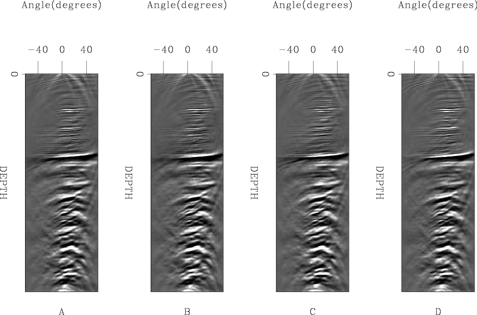
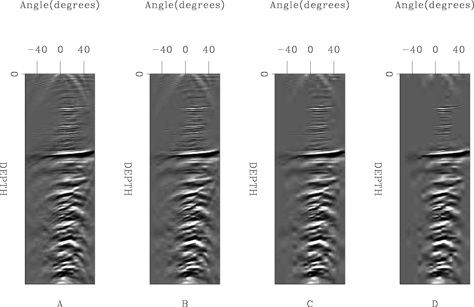
We get a more interesting result if we look at the compressibility of angle gathers. Figure 5 shows the same locations as Figure 2 but in the angle domain. Figure 6 shows the resulting wavelet domain space and a histogram of its absolute values. Note an even greater clustering around 0. Figure 7 shows the result of thresholding the wavelet domain at 95%, 98%, 99%, 99.5%. Note how we see near perfect reconstruction of the angle gather up to 99% and potential up to 99.5%. This is a 100:1 to 200:1 compression ratio (which translates into 20 to 50x reduction in sub-surface offsets).
Framing the compression in terms of angle gathers requires a change in formulation.
The ![]() in equation 2 now becomes chain of two operators.
The first translates from sub-surface offset to angle. The second is multi-dimensional
wavelet transform.
in equation 2 now becomes chain of two operators.
The first translates from sub-surface offset to angle. The second is multi-dimensional
wavelet transform.
|
|---|
|
angle
Figure 5. Four angle gathers at the same locations seen in Figure 2. |
|
|

|
|---|
|
wavelet2
Figure 6. Panel A shows the wavelet domain representation of the 4-D volume used in this experiment transformed into the angle domain. Panel B shows a poriton of the wavelet domain. Panel C shows a histogram of the wavelet domain values. Note how the vast majority of the values are nearly zero. |
|
|
|
|---|
|
angle2
Figure 7. The result of zeroing the smallest values of the wavelet domain representation shown in Figure 3A. All four panels show the same sub-surface offset gather shown in Figure 5. A shows the result of clipping 95% of the values; B, 98%; C, 99%; and D,99.5%. Note how the reconstructed gather is nearly identical up to a 99% clip. |
|
|
|
|
|
|
Imaging using compressive sensing |