|
|
|
|
Imaging using compressive sensing |
Until recently, a zero-time, zero-subsurface offset imaging condition
was the most commonly implemented method. This amounts producing an image ![]() by
by
| (3) |
 the cost of our finite
difference stencil. As of this writing, we are nearing a cross-over point where
this will no longer be valid.
the cost of our finite
difference stencil. As of this writing, we are nearing a cross-over point where
this will no longer be valid.
The relative cost of implementing the actual imaging
condition is a little trickier. For this exercise, let's assume that we are implementing
acoustic RTM on a GPGPU (the relatively simple memory model simplifies the calculation).
Let's assume a naive second-order in time, 14th order in space approach. In this
case, at each sample we need to read in the previous wavefield, the velocity, and store the
updated wavefield. In addition, we will access 43 values in the current wavefield, but because
these are stored in shared memory they will have approximately
![]() latency.
Therefore, the cost of propagating the wavefield eight times between imaging steps will be
latency.
Therefore, the cost of propagating the wavefield eight times between imaging steps will be
![]() . The imaging step at each point will require the reading of
the source and receiver wavefield from global memory, and the reading and writing of
the image, a cost of
. The imaging step at each point will require the reading of
the source and receiver wavefield from global memory, and the reading and writing of
the image, a cost of
![]() , or a magnitude less than the propagation cost.
, or a magnitude less than the propagation cost.
Alternate imaging condition choices such as offset-gathers(Sava and Fomel, 2003),
time-shift gathers(Sava and Fomel, 2006),
and extended image gathers(Sava, 2007), dramatically alter this balance. For conciseness I will
limit this discussion to sub-surface offset gathers, but similar limitations apply to
all of the choices. To construct sub-surface offset gathers used to form angle gathers, the
image, in its most general form, expands by one to three dimensions.
In the extreme case, the image becomes
![]() ,
where
,
where ![]() and
and ![]() represent lags in
represent lags in ![]() and
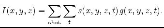
and ![]() . The imaging condition
then becomes
. The imaging condition
then becomes
| (4) |
 ) to several thousand times larger. As a result,
it must now be read and written to disk at every imaging step. If we assume that we
are constructing 400 sub-surface offsets at each point, the computational cost increases
dramatically. We now benefit from transferring the source and receiver wavefields to shared
memory, reducing their cost by possibly up to 80%, but we still end up with a cost
of
) to several thousand times larger. As a result,
it must now be read and written to disk at every imaging step. If we assume that we
are constructing 400 sub-surface offsets at each point, the computational cost increases
dramatically. We now benefit from transferring the source and receiver wavefields to shared
memory, reducing their cost by possibly up to 80%, but we still end up with a cost
of
Sub-sampling sub-surface offsets offers benefits in both computation and storage. The reduction in offset calculation proportionally reduces the storage on large memory machines, potentially eliminating the need to go to disk. Total computation is reduced by sub-sampling, but given the required random nature of compressive sensing, cache misses will not be proportionally reduced.
|
|
|
|
Imaging using compressive sensing |