Tests of orthogonalization

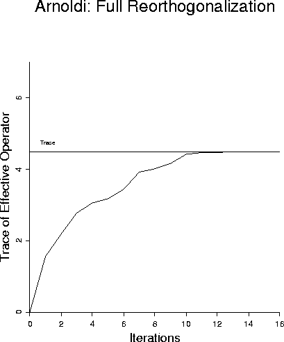
For the LSQR algorithm, it is easy to check the trace of the effective operator since it is just the sum of the squares of the elements in the resulting bidiagonal matrix. To test the ideas of the preceding section, we first perform an LSQR inversion while imposing full reorthogonalization Arnoldi (1951) at each step. Doing so, we obtain Figure 5, showing that the effective operator trace converges monotonically to the true trace from below as expected.

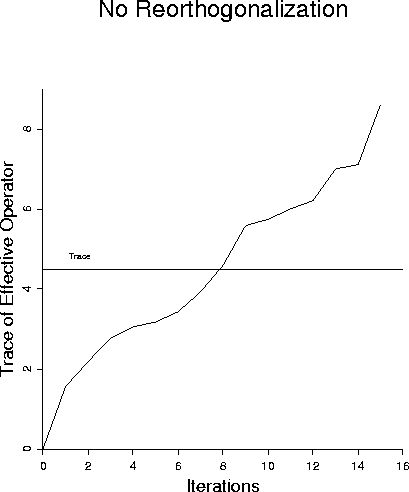
In contrast, Figure 6 shows that without reorthogonalization the trace of the effective operator has already exceeded the upper bound -- thus demonstrating that the eighth direction vector found by LSQR has at least some component parallel to one of the earlier vectors and also along some eigenvector with large eigenvalue. Observing the later behavior of this curve, regions of small slopes may correspond to allowable (orthogonal) direction vectors, but the regions of large slope must be resampling the regions of the vector space with the largest eigenvalues. This observation shows that the rebirth of nonorthogonal vectors does not happen just at the eighth iteration, but is a recurring problem.

These two examples show clearly that full reorthogonalization works very well and that failure to do any reorthogonalization can lead to serious problems with the set of direction vectors generated by such schemes. To make progress, we want to know whether full reorthogonalization is required, or whether some type of partial reothogonalization (which will presumably be cheaper) might be equally or almost as effective as full reorthogonalization. We want to explore the tradeoffs between cost of the partial reorthogonalization and the benefits to be derived from it. Figures 7-11 explore these issues.

 

sumarnoldi
Figure 5 LSQR with full (Arnoldi) reorthogonalization.

 

sum000
Figure 6 LSQR with no reorthogonalization.

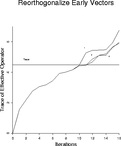
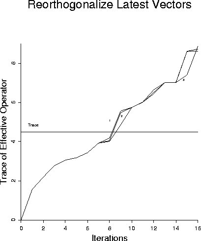
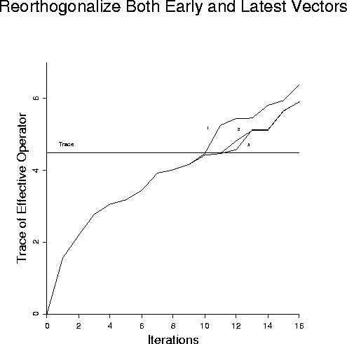
Figures 7-9 refer to the same model considered in Figures 1-6. Figure 7 shows that orthogonalizing against the first 1, 2, or 3 vectors improves the results progressively, the more vectors are used for the reorthogonalization. Figure 8 shows that reorthogonalization against the 1, 2, or 3 most recently generated vectors does not work as well as the previous Figure. Reorthogonalizing against both 1, 2, or 3 early and late vectors gives virtually identical results in Figure 9 as those results observed in Figure 7.

 

sum310
Figure 7 LSQR with partial reorthogonalization - first one, two, or three.

 

sum301
Figure 8 LSQR with partial reorthogonalization - last one, two, or three.

 

sum311
Figure 9 LSQR with partial reorthogonalization - using both first and last one, two, or three.

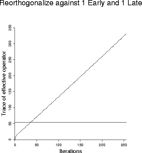
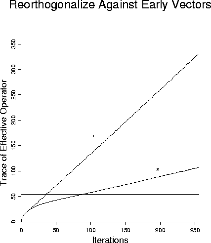
Figures 10 and 11 refer to a model of $16\times8$ cells similar to that considered earlier by Berryman 1990. Figure 10 shows that reorthogonalizing against only the first and last vectors generated in the iteration sequence is quite ineffective at reducing the nonorthogonal vectors generated. Figure 11 shows that reorthogonalizing against the first 35 vectors produces a major improvement, without significant orthogonalization problems out to 90 iterations, instead of less than 35 iterations before problems arise with only one vector reothogonalization.

 

ex111
Figure 10 LSQR with partial reorthogonalization - using first and last vector.

 

ex3510
Figure 11 LSQR with partial reorthogonalization - using first or first 35 vectors.

We conclude that reorthogonalization is effective and the partial reorthogonalization is most effective when the vectors chosen for the reorthogonalization set are those from the early part of the iteration sequence. The reason that these vectors are best to use is presumably because they correspond to directions that have components parallel to directions in the space that are eigenvectors of the operator being inverted with largest eigenvalues. These vectors like to be reborn in this process and reorthogonalization is an effective means of preventing multiply copies of the same dominant vectors from recurring in the iteration sequence.