

Next: Seismic field data examples
Up: PREDICTION-ERROR FILTER OUTPUT IS
Previous: PEF whiteness proof in
Here we examine elementary signal-processing applications of
2-D prediction-error filters (PEFs)
on both everyday 2-D textures and on seismic data.
Some of these textures are easily modeled with
prediction-error filters (PEFs) while others are not.
All figures used the same  filter shape.
No attempt was made to optimize filter size
or shape or any other parameters.
Results in Figures
![[*]](http://sepwww.stanford.edu/latex2html/cross_ref_motif.gif) -
-![[*]](http://sepwww.stanford.edu/latex2html/cross_ref_motif.gif) are shown with various familiar textures
are shown with various familiar textures![[*]](http://sepwww.stanford.edu/latex2html/foot_motif.gif) on the left
as training data sets.
From these training data sets,
a prediction-error filter (PEF) is estimated
using module pef
on the left
as training data sets.
From these training data sets,
a prediction-error filter (PEF) is estimated
using module pef ![[*]](http://sepwww.stanford.edu/latex2html/cross_ref_motif.gif) .
The center frame is simulated data made by deconvolving
(polynomial division) random numbers by the estimated PEF.
The right frame is the more familiar process,
convolving the estimated PEF on the training data set.
.
The center frame is simulated data made by deconvolving
(polynomial division) random numbers by the estimated PEF.
The right frame is the more familiar process,
convolving the estimated PEF on the training data set.
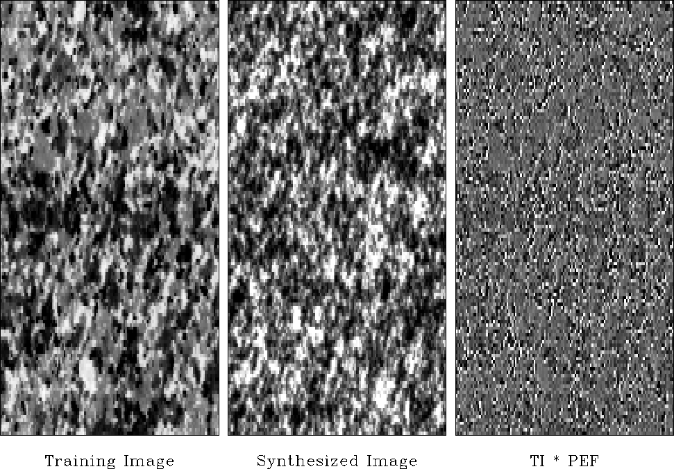
granite
Figure 3
Synthetic granite matches the training image quite well.
The prediction error (PE) is large at grain boundaries
so it almost seems to outline the grains.


Theoretically, the right frame tends towards a white spectrum.
Earlier you could notice
the filter size by knowing that the output
was taken to be zero where the filter is only partially on the data.
This was annoying on real data where we didn't want to throw
away any data around the sides.
Now the filtering is done without a call to the boundary module
so we have typical helix wraparound.
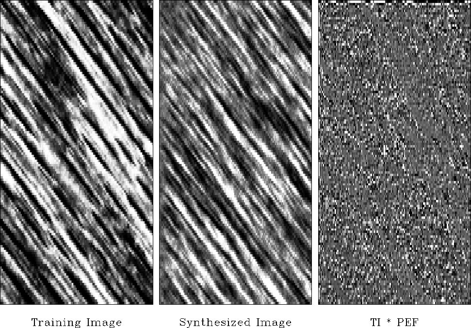
wood
Figure 4
Synthetic wood grain has too little white.
This is because of the nonsymmetric brightness histogram of natural wood.
Again, the PEF output looks random as expected.


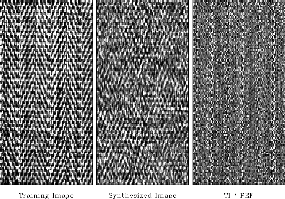
herr
Figure 5
A banker's suit (left). A student's suit (center). My suit (right).
The prediction error is large where the weave changes direction.


basket
Figure 6
Basket weave.
The simulated data fails to segregate the two dips into a checkerboard pattern.
The PEF output looks structured perhaps because the filter is too small.


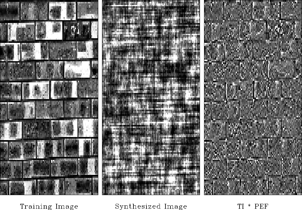
brick
Figure 7
Brick.
Synthetic brick edges are everywhere
and do not enclose blocks containing a fixed color.
PEF output highlights the mortar.


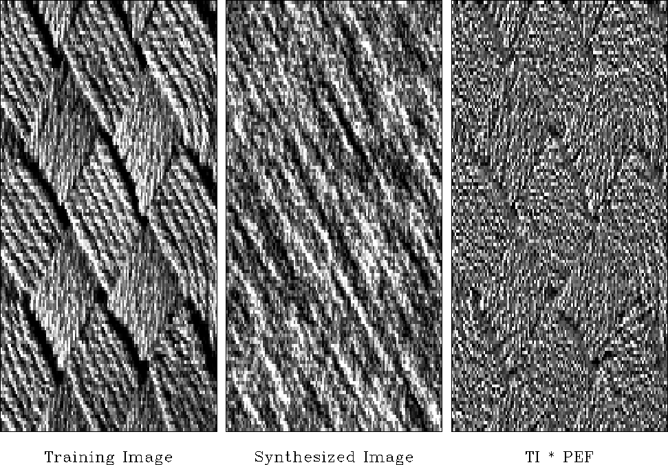
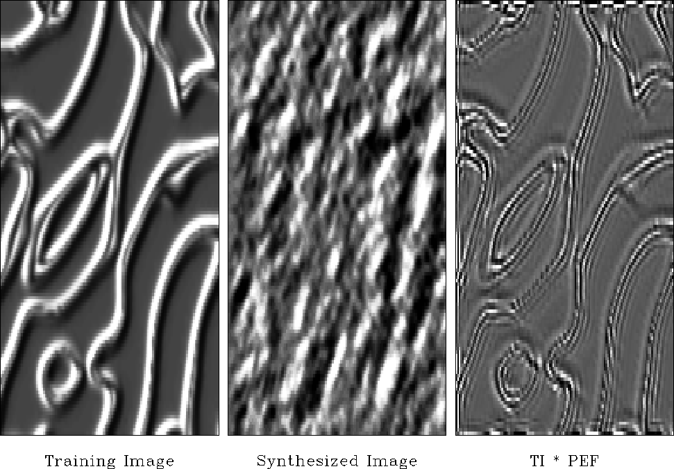
ridges
Figure 8
Ridges.
A spectacular failure of the stationarity assumption.
All dips are present but in different locations.
Never-the-less,
the ridges have been sharpened by the deconvolution.


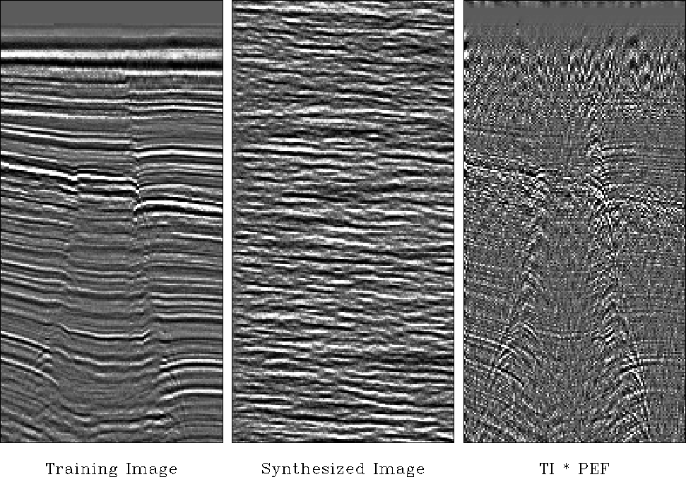
WGstack
Figure 9
Gulf of Mexico seismic section, modeled, and deconvolved.
Do you see any drilling prospects in the simulated data?
In the deconvolution, the strong horizontal layering
is suppressed giving a better view of the hyperbolas.
The decon filter is the same  used on the everyday textures.


Since a PEF tends to the inverse of the spectrum of its input,
results similar to these could probably be found
using Fourier transforms, smoothing spectra, etc.
We used PEFs because of their flexibility.
The filters can be any shape.
They can dodge around missing data, or we can use them
to estimate missing data.
We avoid periodic boundary assumptions inherent to FT.
The PEF's are designed only internal to known data, not off edges
so they are readily adaptible to nonstationarity.
Thinking of these textures as seismic time slices,
the textures could easily be required to pass thru specific
values at well locations.


Next: Seismic field data examples
Up: PREDICTION-ERROR FILTER OUTPUT IS
Previous: PEF whiteness proof in
Stanford Exploration Project
4/27/2004
![[*]](http://sepwww.stanford.edu/latex2html/cross_ref_motif.gif) -
-![[*]](http://sepwww.stanford.edu/latex2html/cross_ref_motif.gif) are shown with various familiar textures
are shown with various familiar textures![[*]](http://sepwww.stanford.edu/latex2html/foot_motif.gif) on the left
as training data sets.
From these training data sets,
a prediction-error filter (PEF) is estimated
using module pef
on the left
as training data sets.
From these training data sets,
a prediction-error filter (PEF) is estimated
using module pef ![[*]](http://sepwww.stanford.edu/latex2html/cross_ref_motif.gif) .
The center frame is simulated data made by deconvolving
(polynomial division) random numbers by the estimated PEF.
The right frame is the more familiar process,
convolving the estimated PEF on the training data set.
.
The center frame is simulated data made by deconvolving
(polynomial division) random numbers by the estimated PEF.
The right frame is the more familiar process,
convolving the estimated PEF on the training data set.
