ALTITUDE OF SEA SURFACE NEAR MADAGASCAR

A satellite points a radar at the ground and receives echos we investigate here. These echos are recorded only over the ocean. The echo tells the distance from the orbit to the ocean surface. After various corrections are made for earth and orbit ellipticities the residual shows tides, wind stress on the surface, and surprisingly a signal proportional to the depth of the water. Gravity of mountains on the water bottom pulls water towards them raising sea level there.

The raw data investigated here had a strong north-south tilt which I removed at the outset. Figure  gives our first view of altimetry data (ocean height) from southeast of the island of Madagascar.

 

jesse1
Figure 9 Sea height under satellite tracks. The island of Madagascar is in the empty area at $(46^\circ,-22^\circ)$. Left is the adjoint $\bold L'\bold d$. Right is the adjoint normalized by the bin count, ${\bf diag}(\bold L'\bold 1)^{-1} \bold L'\bold d$. You might notice a few huge, bad data values. Overall, the topographic function is too smooth, suggesting we need a roughener.

About all we can see is satellite tracks. The satellite is in a circular polar orbit. To us the sun seems to rotate east to west as does the circular satellite orbit. Consequently, when the satellite moves northward across the site we get altitude measurements along a SE-NW line. When it moves southward we get measurements along a NE-SW line. This data is from the cold war era. At that time dense data above the $-30^\circ$ parallel was secret although sparse data was available. (The restriction had to do with precision guidance of missiles. Would the missile hit the silo? or miss it by enough to save the retaliation missile?)

Here are some definitions: Let components of $\bold d$ be the data, altitude measured along a satellite track. The model space is $\bold h$, altitude in the (x,y)-plane. Let $\bold L$ denote the 2-D linear interpolation operator from the track to the plane. Let $\bold H$ be the helix derivative, a filter with response $\sqrt{k_x^2+k_y^2}$.Except where otherwise noted, the roughened image $\bold p$ is the preconditioned variable $\bold p =\bold H \bold h$.The derivative along a track in data space is ${d\over dt}$.A weighting function that vanishes when any filter hits a track end or a bad data point is $\bold W$.

 

jesse5
Figure 10 All the data $\bold d$ and the missing data markers.

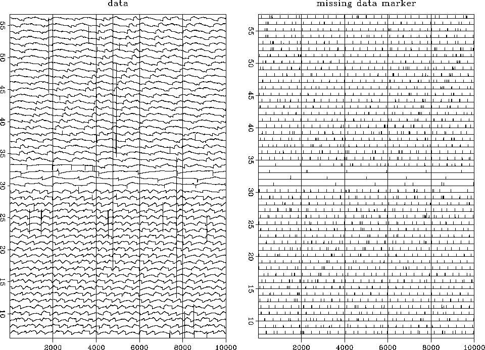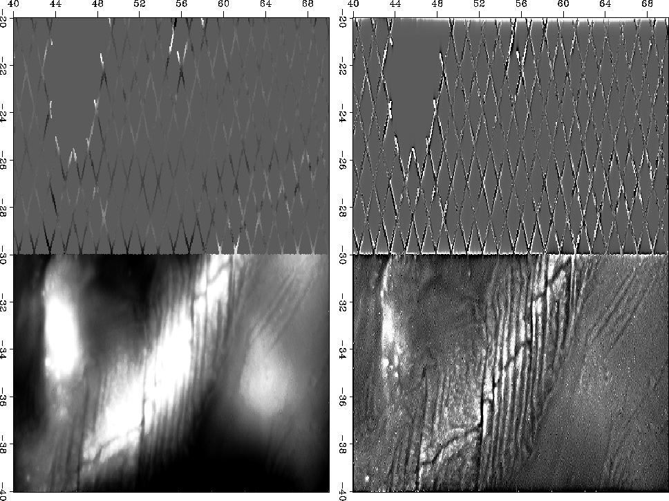
Figure  shows the entire data space, over a half million data points (actually 537974). Altitude is measured along many tracks across the image. In Figure  the tracks are placed end-to-end, so it is one long vector (displayed in about 50 signal rows). A vector of equal length is the missing data marker vector. This vector is filled with zeros everywhere except where data is missing or known bad or known to be at the ends of the tracks. The long tracks are the ones that are sparse in the north.

 

jesse2 Figure 11 The roughened, normalized adjoint, 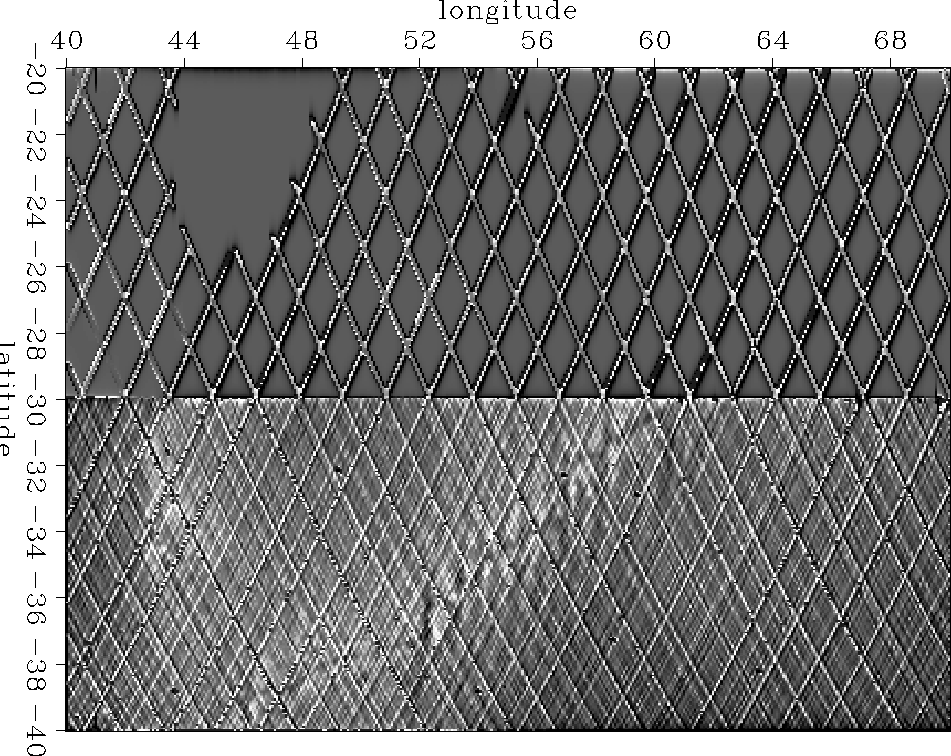$\bold H \ {\bf diag}(\bold L'\bold 1)^{-1} \bold L'\bold d$. Some topography is perceptible through a maze of tracks.

Figure  brings this information into model space. Applying the adjoint of the linear interpolation operator $\bold L'$to the data $\bold d$ gave our first image $\bold L'\bold d$in model space in Figure . The track noise was so large that roughening it made it worse. A more inviting image arose when I normalized the image before roughening it. Put a vector of all ones $\bold 1$ into the adjoint of the linear interpolation operator $\bold L'$.What comes out $\bold L'\bold 1$is roughly the number of data points landing in each pixel in model space. More precisely, it is the sum of the linear interpolation weights. This then, if it is not zero, is used as a divisor. The division accounts for several tracks contributing to one pixel. In matrix formalism this image is ${\bf diag}(\bold L'\bold 1)^{-1} \bold L'\bold d$.In Figure  this image is roughened with the helix derivative $\bold H$.

 

jesse3
Figure 12 With a simple roughening derivative in data space, model space shows two nice topographic images. Let $\bold n$ denote ascending tracks. Let $\bold s$ denote descending tracks. Left is $\bold L' {d\over dt} \bold n$. Right is $\bold L' {d\over dt} \bold s$.

There is a simple way here to make a nice image--roughen along data tracks. This is done in Figure . The result is two attractive images, one for each track direction. Unfortunately, there is no simple relationship between the two images. We cannot simply add them because the shadows go in different directions. Notice also that each image has noticeable tracks that we would like to suppress further.

A geological side note: The strongest line, the line that marches along the image from southwest to northeast is a sea-floor spreading axis. Magma emerges along this line as a source growing plates that are spreading apart. Here the spreading is in the north-south direction. The many vertical lines in the image are called ``transform faults''.

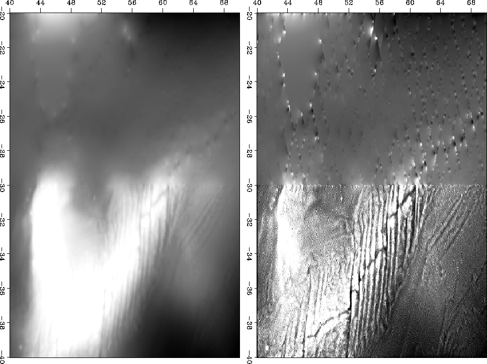
Fortunately, we know how to merge the data. The basic trick is to form the track derivative not on the data (which would falsify it) but on the residual which (in Fourier space) can be understood as choosing a different weighting function for the statistics. A track derivative on the residual is actually two track derivatives, one on the observed data, the other on the modeled data. Both data sets are changed in the same way. Figure  shows the result.

 

jesse10
Figure 13 All data merged into a track-free image (hooray!) by applying the track derivative, not to the data, but to the residual. Left is $\bold h$ estimated by $\bold 0\approx \bold W {d\over dt}(\bold L\bold h-\bold d)$. Right is the roughened altitude, $\bold p =\bold H \bold h$.

The altitude function remains too smooth for nice viewing by variable brightness, but roughening it with $\bold H$ makes an attractive image showing, in the south, no visible tracks.

The north is another story. We would like the sparse northern tracks to contribute to our viewing pleasure. We would like them to contribute to a northern image of the earth, not to an image of the data acquisition footprint.

 

jesse8
Figure 14 Using the track derivative in residual space and helix preconditioning in model space we start building topography in the north. Left is $\bold h=\bold H^{-1}\bold p$ where $\bold p$ is estimated by $\bold 0 \approx \bold W {d\over dt} (\bold L\bold H^{-1}\bold p-\bold d)$ for only 10 iterations. Right is $\bold p =\bold H \bold h$.

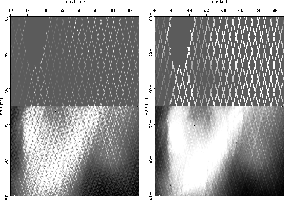
This begins to happen in Figure . The process of fitting data by choosing an altitude function $\bold h$would normally include some regularization (model styling), such as $\bold 0\approx \nabla \bold h$.Instead we adopt the usual trick of changing to preconditioning variables, in this case $\bold h=\bold H^{-1}\bold p$.As we iterate with the variable $\bold p$ we watch the images of $\bold h$ and $\bold p$ and quit either when we are tired, or more hopefully, when we are best satisified with the image. This subjective choice is rather like choosing the $\epsilon$that is the balance between data fitting goals and model styling goals. The result in Figure  is pleasing. We have begun building topography in the north that continues in a consistant way with what is in the south. Unfortunately, this topography does fade out rather quickly as we get off the data acquisition tracks.

If we have reason to suspect that the geological style north of the 30th parallel matches that south of it (the stationarity assumption) we can compute a PEF on the south side and use it for interpolation on the north side. This is done in Figure .

 

jesse9
Figure 15 Given a PEF $\bold A$ estimated on the densely defined southern part of the model, $\bold p$ was estimated by $\bold 0\approx \bold W {d\over dt}(\bold L\bold A^{-1}\bold p-\bold d)$ for 50 iterations. Left is $\bold h = \bold A^{-1}\bold p$. Right is $\bold p =\bold H \bold h$.

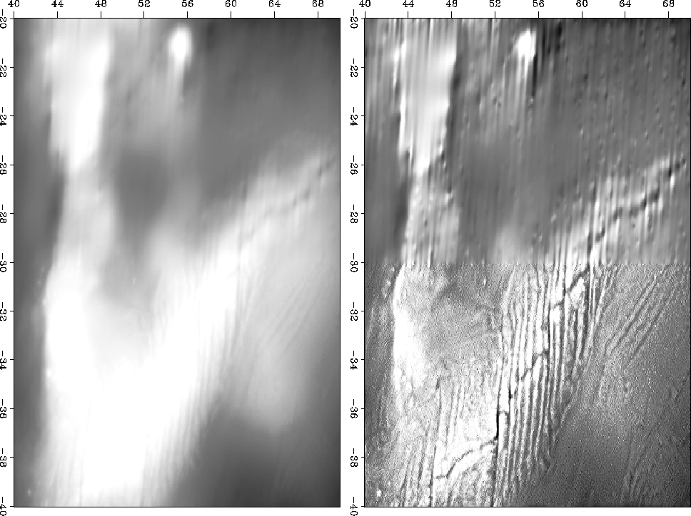This is about as good as we are going to get. Our fractured ridge continues nicely into the north. Unfortunately, we have imprinted the fractured ridge texture all over the northern space, but that's the price we must pay for relying on the stationarity assumption.

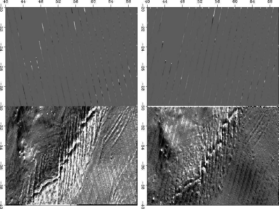
The fitting residuals are shown in Figure .

 

jesse9_res
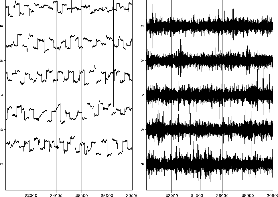Figure 16 The residual at fifty thousand of the half million (537,974) data points in Figure . Left is physical residual $\bold L\bold A^{-1}\bold p -\bold d$. Right is fitting residual $\bold W {d\over dt} (\bold L\bold A^{-1}\bold p -\bold d)$.

The physical altitude residuals tend to be rectangles, each the duration of a track. While the satellite is overflying other earth locations the ocean surface is changing its altitude. The fitting residuals (right side) are very fuzzy. They appear to be ``white'', though with ten thousand points crammed onto a line a couple inches long, we cannot be certain. We could inspect this further. If the residuals turn out to be significantly non-white, we might do better to change ${d\over dt}$ to a PEF along the track.