Beam Stack Inversion

In this paper I formulate the beam stack inversion as an iterative least squares problem in the frequency domain. I use a conjugate gradient solver to find the model, $\bf m$, that minimizes the residual, $\bf r$, in the following system:

$$\begin{eqnarray} \bf r &=& \bf \vert\vert(d-Hm)\vert\vert^2\end{eqnarray}$$ (6)

In my previous work with Biondi, we formulated the iterative problem in the time domain. As opposed to the iterative time domain representation, the frequency domain formulation is appreciably faster.

 

nmo
Figure 6 NMO-corrected synthetic data.

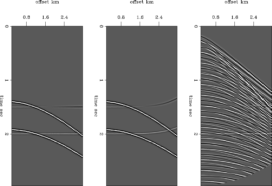
I applied the inversion to the synthetic data displayed in figure after applying NMO. The NMO-corrected synthetic data is displayed in figure . The application of NMO has the effect of limiting the dip range in the data. This reduces the size of the model space necessary to represent the input data.

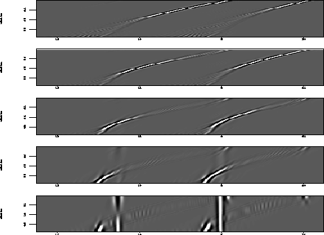
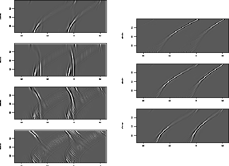
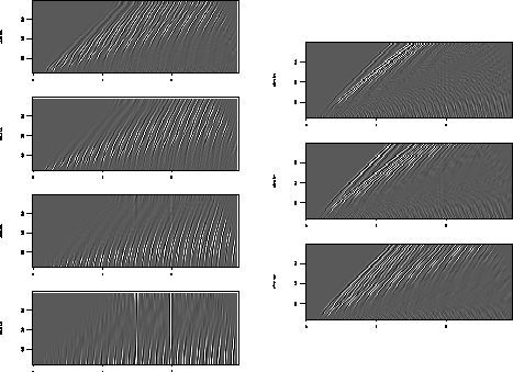
The inversion results for the NMO-corrected data appear in figures , + . Each figure displays all the slowness slices from the model space of the beam stack inversion. It is apparent from figures + that the primary energy is confined to the zero slowness slice of the model space, while figure shows that the primary energy resides in zero and negative slowness slices.

 

invnmo1
Figure 7 Inversion of NMO-corrected model1. The slices displayed from bottom to top have the following constant slowness values(s/km): p₁=0.0,p₂=0.075,p₃=0.15,p₄=0.225,p₅=0.3

 

invnmo2
Figure 8 Inversion of NMO-corrected model2. The slices displayed from bottom-left to top-right have the following constant slowness values(s/km): p₁=-0.15,p₂=-0.075,p₃=-0.0,p₄=0.075,p₅=0.15,p₆=0.225,p₇=0.3

 

invnmo3
Figure 9 Inversion of NMO-corrected model3. The slices displayed from bottom-left to top-right have the following constant slowness values(s/km): p₁=0.0,p₂=0.075,p₃=0.15,p₄=0.225,p₅=0.3,p₆=0.375,p₇=0.45

I forward modeled each inversion result to produce a reconstruction of the NMO-corrected synthetic data. The difference in total energy between the reconstructed synthetic data and original synthetic data is less than $2\%$ in each case. This difference was achieved in five iterations and required three minutes of computing time on one processor of an SGI power challenge.

An alternative to the iterative least-squares solution is a direct inversion. To implement the direct inversion, the data covariance matrix, $\bf{HH^{\dagger}}$, must be inverted. This matrix, and the beam stack operator itself, can be partitioned into a separate matrix for each frequency of interest, thus reducing the size of the data covariance matrix significantly. The partitioned beam stack operator in matrix form is of size (N_x)(N_xN_p) while the partitioned data covariance matrix is of size (N_x)(N_x). In order to apply a direct least squares inversion, the data covariance matrix would have to be inverted for each frequency of interest and applied as a pre-conditioner to the application of the adjoint to the data.

Hampson (1986) used this approach to formulate the direct least squares inverse of the parabolic radon transform. In the case of the radon transform, the model covariance matrix must be inverted. The model covariance matrix of the PRT is of size (N_p)(N_p) where p is the slowness parameter of the PRT. A typical range of the PRT parameter p is 50. Kostov (1990) has shown that the family of radon transforms results in a model covariance matrix that is Toeplitz in structure and as such can be inverted with the Levinson method (and other methods) at a cost proportional to n² instead of n³, where n is the size of the matrix to be inverted Claerbout (1976). The Toeplitz property of the PRT model covariance matrix coupled with its reasonable size, around, $50\times 50$, elements, make a direct inversion of the PRT model covariance matrix reasonable. The parabolic beam stack data covariance matrix is not Toeplitz and it's size is equal to the square of the number of offsets in the data. Because of these features, the parabolic beam stack operator is not a great candidate for a direct inversion.