![[*]](http://sepwww.stanford.edu/latex2html/prev_gr.gif)


Next: About this document ...
Up: Table of Contents
0=25
The time and space formulation
of azimuth moveout
Sergey Fomel and Biondo L. Biondi
sergey@sep.stanford.edu, biondo@sep.stanford.edu
ABSTRACT
Azimuth moveout (AMO) transforms 3-D prestack seismic data from one
common azimuth and offset to different azimuths and offsets.
AMO in the time-space domain is represented by a three-dimensional
integral operator. The operator components are the summation path,
the weighting function, and the aperture. To determine the summation path and
the weighting function, we derive the AMO operator by cascading dip
moveout (DMO) and inverse DMO for different azimuths in the time-space
domain. To evaluate the aperture, we apply a geometric approach,
defining AMO as the result of cascading prestack migration (inversion)
and modeling. The aperture limitations provide a consistent
description of AMO for small azimuth rotations (including zero) and justify the
economic efficiency of the method.
|
Azimuth moveout (AMO) is by definition an operator that transforms
common-azimuth common-offset seismic reflection data to different
azimuths and offsets![[*]](http://sepwww.stanford.edu/latex2html/foot_motif.gif) . A constructive approach to
AMO was proposed by Biondi and Chemingui
. According to this approach, an AMO
operator is built by cascading the dip moveout (DMO) operator that
transforms the input common-azimuth data to zero offset, and the inverse
DMO that transforms the zero-offset data to a new offset and azimuth.
Evaluating the cascade of the frequency-domain DMO and inverse DMO
operators by means of the stationary phase technique produces the
integral (Kirchhoff-type) 3-D AMO operator in the time-space domain.
. A constructive approach to
AMO was proposed by Biondi and Chemingui
. According to this approach, an AMO
operator is built by cascading the dip moveout (DMO) operator that
transforms the input common-azimuth data to zero offset, and the inverse
DMO that transforms the zero-offset data to a new offset and azimuth.
Evaluating the cascade of the frequency-domain DMO and inverse DMO
operators by means of the stationary phase technique produces the
integral (Kirchhoff-type) 3-D AMO operator in the time-space domain.
The first part of this paper applies an analogous idea to construct the AMO
operator from the time-space domain DMO and
achieves the same result in a simpler way.
Cascading DMO and inverse DMO allows us to evaluate the AMO operator's
summation path and the corresponding weighting function. However, it
is not sufficient for evaluating the third major component of the
integral operator, that is, its aperture (range of integration). To solve this
problem, we apply an
alternative approach, that
defines AMO as a cascade of 3-D migration (inversion) for
particular common-azimuth
and common-offset data and 3-D modeling for a different azimuth and
offset. This
definition resembles the viewpoint on DMO developed by Deregowski and Rocca
. As with the DMO case, the
migration and modeling approach reveals the physics of the AMO
aperture and limits its boundaries.
It is the aperture limitation
that allows us to overcome the paradoxical inconsistency between 2-D
and 3-D AMO operators discussed by Biondi and Chemingui
.
If the aperture is chosen properly, the AMO operator converges to the 2-D
offset continuation limit as the azimuth rotation approaches zero.
This remarkable fact supports the proof of economical
efficiency of AMO in comparison with the prestack migration operator,
which is known to have an unlimited aperture.
CASCADING DMO AND INVERSE DMO
IN TIME-SPACE DOMAIN
In this section, we present a new version of the AMO derivation.
Since
the entire derivation is performed in the time-space domain, it is more
straightforward than the stationary phase technique developed for the
same purpose by Biondi and Chemingui .
Let  be the input of an AMO
operator (common-azimuth and common-offset seismic
reflection data after normal moveout correction) and
be the input of an AMO
operator (common-azimuth and common-offset seismic
reflection data after normal moveout correction) and
 be the output. Here
 are midpoint locations on the surface:
 , and
, and
 are half-offset vectors.
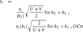
The 3-D AMO operator has the following general form:
are half-offset vectors.
The 3-D AMO operator has the following general form:
|  |
(1) |
where  is the differentiation operator
  ,
,  is the summation
path, and w12 is the weighting function. In this section we will
evaluate
is the summation
path, and w12 is the weighting function. In this section we will
evaluate  and w12 using the cascade of integral 3-D DMO and
inverse DMO operators in the time-space domain. The idea of this
derivation originated in Biondi and Chemingui's paper
, where it was
applied with the frequency-domain DMO and inverse DMO operators. In
the next section,
we apply a new geometric approach to evaluate the AMO aperture (range of
integration in AMO).
and w12 using the cascade of integral 3-D DMO and
inverse DMO operators in the time-space domain. The idea of this
derivation originated in Biondi and Chemingui's paper
, where it was
applied with the frequency-domain DMO and inverse DMO operators. In
the next section,
we apply a new geometric approach to evaluate the AMO aperture (range of
integration in AMO).
To derive AMO in the time-space domain,
an integral
(Kirchoff-type) DMO operator of the form
|  |
(2) |
is cascaded with an inverse DMO of the form
|  |
(3) |
where  stands for the operator of half-order differentiation
(equivalent to
stands for the operator of half-order differentiation
(equivalent to  multiplication in Fourier domain),
 and
and  are the summation paths of
the DMO and inverse DMO
operators ():
are the summation paths of
the DMO and inverse DMO
operators ():
|  |
(4) |
| (5) |
w10 and w02 are the corresponding weighting functions (amplitudes of
impulse responses),  is the component of
  along the
 azimuth, and
  is the component of
  along the
 azimuth.
Integral operators DMO and IDMO correspond to
the high-frequency asymptotic (the geometrical seismic) description of
the wave field. As shown by Stovas and Fomel ,
operator IDMO has an asymptotically equivalent
form
azimuth.
Integral operators DMO and IDMO correspond to
the high-frequency asymptotic (the geometrical seismic) description of
the wave field. As shown by Stovas and Fomel ,
operator IDMO has an asymptotically equivalent
form
|  |
(6) |
where  .
.
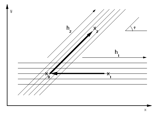
Both DMO and inverse DMO operate on 3-D seismic data
as 2-D operators, since their apertures are defined on a line. This
implies that for a given input midpoint , the corresponding
location of must belong to the
line going through , with the azimuth defined by the input
offset .
Similarly, must be on the line going through
 with the azimuth of (Figure amox12).
These theoretical facts lead us to the following conclusion:
with the azimuth of (Figure amox12).
These theoretical facts lead us to the following conclusion:
For a given pair of input and output midpoints and of the AMO operator, the corresponding midpoint on
the intermediate zero-offset gather is determined by the intersection of
two lines drawn
through and in the offset directions.
Applying the geometric connection among the three midpoints, we can
find the cascade
of the DMO
and inverse DMO operators in one step.
For this purpose, it is convenient to choose an orthogonal coordinate
system  on the
surface in such a way that the direction of the x axis corresponds
to the input azimuth
(Figure amox12).
In this case the connection between the three midpoints is given by
on the
surface in such a way that the direction of the x axis corresponds
to the input azimuth
(Figure amox12).
In this case the connection between the three midpoints is given by
|  |
(7) |
| (8) |
amox12
Figure 1 Geometric
relationships between input and output midpoint locations in AMO.

Substituting DMO into tIDMO and taking into account
jacob produces the 3-D integral AMO operator AMO,
where
| 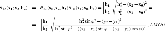 |
|
| (9) |
|  |
(10) |
 . Equation
 is the same
as equation (4) in () except for a different
notation. The weighting function of the derived AMO operator
is the same
as equation (4) in () except for a different
notation. The weighting function of the derived AMO operator
 depends on the weighting functions of DMO and inverse DMO that are involved in
the construction. In Appendix A, we apply equation AMOwf to two
popular versions of the DMO weighting functions that
correspond to Hale's and Zhang's
DMO operators.
depends on the weighting functions of DMO and inverse DMO that are involved in
the construction. In Appendix A, we apply equation AMOwf to two
popular versions of the DMO weighting functions that
correspond to Hale's and Zhang's
DMO operators.
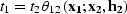
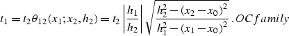
Deriving formula AMOtt, we have to assume
that the input
and output offset azimuths are different ( ). In the case
of equal azimuths, AMO reduces to 2-D offset continuation (OC). The
location of in this case is not constrained by the input
and output midpoints and can take different values on the line.
Therefore the superposition of DMO and inverse DMO for offset
continuation is a convolution on that line. To find the summation path
of the OC operator, we should consider the envelope of the family of traveltime
curves (where x0 is the parameter of a curve in the family):
). In the case
of equal azimuths, AMO reduces to 2-D offset continuation (OC). The
location of in this case is not constrained by the input
and output midpoints and can take different values on the line.
Therefore the superposition of DMO and inverse DMO for offset
continuation is a convolution on that line. To find the summation path
of the OC operator, we should consider the envelope of the family of traveltime
curves (where x0 is the parameter of a curve in the family):
|  |
(11) |
Solving the envelope condition
| 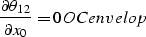 |
(12) |
with respect to x0 produces
|  |
(13) |
where  .Substituting OCx0 into OCfamily, we get the explicit
expression of the OC summation path:
.Substituting OCx0 into OCfamily, we get the explicit
expression of the OC summation path:
|  |
|
| |
| (14) |
where 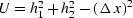 , and
, and
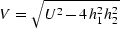 .Equation OCtt corresponds to formula (6) in
() (with a typo corrected). The same
expression was obtained in a different way by Stovas and Fomel
.
The apparent difference between the 2-D and 3-D solutions introduces the
problem of finding a consistent description valid for both cases.
Such a description is especially important for practical applications
dealing with small angles of azimuth rotation, e.g. cable feather
correction in marine seismics. The next section develops
a way of solving
this problem, which
refers to the kinematic theory of AMO and follows the ideas that
Deregowski and Rocca applied
to DMO-type operators.
.Equation OCtt corresponds to formula (6) in
() (with a typo corrected). The same
expression was obtained in a different way by Stovas and Fomel
.
The apparent difference between the 2-D and 3-D solutions introduces the
problem of finding a consistent description valid for both cases.
Such a description is especially important for practical applications
dealing with small angles of azimuth rotation, e.g. cable feather
correction in marine seismics. The next section develops
a way of solving
this problem, which
refers to the kinematic theory of AMO and follows the ideas that
Deregowski and Rocca applied
to DMO-type operators.
AMO APERTURE: CASCADING MIGRATION AND MODELING
The impulse response of the AMO operators corresponds to a spike on
the initial constant-offset constant-azimuth gather. Such a spike
can physically occur in the case of a focusing ellipsoidal
reflector whose focuses are coincident with the initial source and
receiver locations (the impulse response of prestack common-offset
migration). Therefore, the impulse response of AMO corresponds
kinematically to a reflection from this ellipsoid. These
considerations allow us to define AMO as the cascade of the 3-D
common-offset common-azimuth migration and the 3-D modeling for a different
azimuth and offset. An analogous point of
view was
developed for the 2-D case
by Deregowski and Rocca .
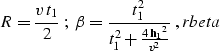
Let's consider the general symmetric ellipsoid equation
|  |
(15) |
where z stands for the depth coordinate, R is the small semi-axis of the
ellipsoid, and  is a nondimensional parameter describing the
stretching of the ellipse
is a nondimensional parameter describing the
stretching of the ellipse  . Deregowski and
Rocca derived the following connections
between the geometric properties of the reflector and the coordinates
of the corresponding spike in the data:
. Deregowski and
Rocca derived the following connections
between the geometric properties of the reflector and the coordinates
of the corresponding spike in the data:
|  |
(16) |
where v is the wave velocity.
The center of the ellipsoid is at the initial midpoint .
This section addresses the kinematic problem of reflection
from the ellipsoid defined by ellips. In particular, we are looking for
the answer to the following question: For a given elliptic
reflector defined by the input midpoint, offset, and time coordinates,
what points on the surface can form a source-receiver pair valid for a
reflection? If a point in the output midpoint-offset space
cannot be related to a reflection pattern, we should exclude it from the AMO
impulse response defined in AMO.
Fermat's principle provides a general method of solving the kinematic reflection problems. Consider a formal expression for the two-point
reflection traveltime
|  |
(17) |
where 
 is the vertical
projection of the reflection
point to the surface,
is the vertical
projection of the reflection
point to the surface,  is the source location, and
 is the receiver location.
According to Fermat's principle, the reflection ray path between two
fixed points must correspond to the
extremum value of the traveltime. Hence, in the vicinity of a
reflected ray,
is the receiver location.
According to Fermat's principle, the reflection ray path between two
fixed points must correspond to the
extremum value of the traveltime. Hence, in the vicinity of a
reflected ray,
| 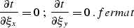 |
(18) |
Solving the system of equations fermat for  and
and  allows us to find the reflection ray path for a given source-receiver
pair on the surface. The solution is derived in Appendix B to be
allows us to find the reflection ray path for a given source-receiver
pair on the surface. The solution is derived in Appendix B to be
|  |
(19) |
|  |
(20) |
where x0 has the same meaning as in the preceding section
and is defined by x012.
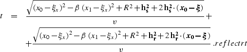
Since the reflection point is contained inside the ellipsoid,
its projection obeys the evident inequality
|  |
(21) |
It is inequality xiyleq that defines the aperture of the AMO
operator.
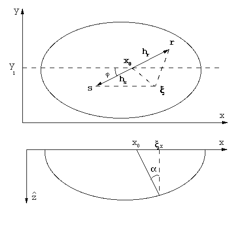
amoapp
Figure 2 The AMO impulse
response traveltime. Parameters:  m,
m,
 m, t1=1 sec. The top plots illustrate
the case of an unrealistically low velocity (v=10 m/s); on the bottom,
v=2000 m/s. On the left side the azimuth rotation
m, t1=1 sec. The top plots illustrate
the case of an unrealistically low velocity (v=10 m/s); on the bottom,
v=2000 m/s. On the left side the azimuth rotation
 ; on the right,


The AMO operator's contours for
different azimuth rotation angles are shown in
Figure amoapp.
Comparing the results for the case of an unrealistically low velocity
(the top two plots in Figure amoapp) and the case of a realistic
velocity (the bottom two plots) clearly demonstrates
the gain in the reduction of the aperture size
achieved by the aperture limitation.
The gain is
especially spectacular for small azimuths. When the azimuth rotation
approaches zero, the area of the 3-D aperture monotonously shrinks to a
line, and the limit of the traveltime of the AMO impulse response
(the inverse of AMOtt) approaches the offset continuation operator
OCtt (Figures amocom). This means that
taking into account
the aperture limitations of AMO provides a consistent description
valid for small azimuth rotations including zero (the offset
continuation case). Obviously, the cost of an integral operator is
proportional to its size. The size of the offset continuation
operator cannot extend the difference between the offsets  . If we applied DMO and
inverse DMO explicitly, the total size of the two operators would be
about
. If we applied DMO and
inverse DMO explicitly, the total size of the two operators would be
about  , which is
substantially greater. This fact proves that in the case of small
azimuth rotations the AMO price is less than those of not only 3-D prestack
migration, but also 3-D DMO and inverse DMO combined ().
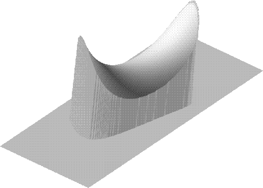
Figure amoavs shows the saddle shape of the AMO operator impulse
response in a 3-D AVS display.
, which is
substantially greater. This fact proves that in the case of small
azimuth rotations the AMO price is less than those of not only 3-D prestack
migration, but also 3-D DMO and inverse DMO combined ().
Figure amoavs shows the saddle shape of the AMO operator impulse
response in a 3-D AVS display.
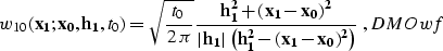
amocom
Figure 3 Traveltime curves
of the impulse responses. The dashed lines indicate the AMO impulse
response with an azimuth rotation of 3 degrees (projection on the x
plane); the solid lines, the 2-D offset continuation impulse response.
|
|  |
amoavs
Figure 4 AMO impulse
response traveltime in three dimensions (the AVS display). Parameters:
m,
m, t1=1 sec, v=2000 m/s,
.
We have applied two different theoretical approaches to AMO to find a
complete definition of the integral
operator AMO. Biondi and Chemingui
proposed cascading the DMO and inverse DMO operators to define AMO in
the frequency domain. The
same approach is repeated here in a simpler way by transferring the
analysis to the natural time-space domain. A new contribution to the
evaluation of the AMO operator follows from applying a different
approach, which extends the geometric theory of DMO
() to the AMO case. Cascading prestack
migration and modeling allows us to evaluate the AMO operator aperture.
The compactness of the AMO aperture indicates that the integral operator can be
performed at a low cost and therefore
promises economic benefits for its practical implementation.
[SEP,EAEG,paper,GEOTLE]
A
AMO AMPLITUDE
The weighting function of the AMO operator can be determined from
cascading the DMO and inverse DMO operators by means of equation
AMOwf. In the case of Hale's DMO () and
its adjoint (),
|  |
(22) |
|  |
(23) |
As follows from HDMOwf,HIDMOwf, and AMOwf,
|  |
(24) |
In the case of the so-called true-amplitude DMO
() and its asymptotic inverse,
|  |
(25) |
|  |
(26) |
Inserting DMOwf and IDMOwf into AMOwf yields
|  |
(27) |
B
DERIVING THE AMO APERTURE
amosym
Figure 5 Reflection from the
ellipsoid of a prestack migration impulse response (a scheme). Top: Map view.
Bottom: Section of the ellipsoid with the plane drawn through the
central line and the reflection point.
|
|  |
This appendix describes the derivation of the main formulas for the
aperture evaluation that follow from the Fermat principle fermat.
In order to avoid the algebraic
complications of fermat, we simplify the
problem by taking into account the cylindrical symmetry of the ellipsoidal
reflector ellips.
Consider a plane drawn through the reflection point and the central line
of the ellipsoid (the axis of the cylindrical symmetry). This plane
has to contain the central (normally reflected) ray from the
reflector. This conclusion follows from the fact that all the normal
reflections emerge at the central line because of the cylindrical
symmetry, as shown in Figure amosym. The intersection of the 3-D
reflector and the plane is the
2-D ellipse
|  |
(28) |
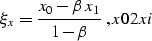
The connection between the emergence point of the normal ray x0 and
the x coordinate of the reflection point can be derived from the
relationship evident in Figure amosym, as follows:
|  |
(29) |
Equation xi2x0 allows us to evaluate in terms of
x0 and get x02xi. The emergence point of the normal ray x0
corresponds to the
midpoint on an imaginary zero-offset section ( with a coincident
source and receiver). Therefore, the location of this point is
determined for given input
and output midpoints in accordance with expression x012.
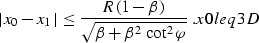
Obviously, the reflection point has to be inside the ellipse
ellips2D. Therefore, its projection obeys the inequality
|  |
(30) |
As follows from xileq, xi2x0, and rbeta,
|  |
(31) |
Inequality x0leq is the known aperture limitation of the DMO
operator DMO found by Deregowski and Rocca
. The equality in x0leq is achieved
when the reflection point is on the surface, where the reflector dip
increases to 90 degrees.
Now the only unknown left in our problem is the y-coordinate of the
reflection point . To find this unknown, we substitute
x02xi into reflecttt, choosing the convenient
parameterization
|  |
(32) |
where  , and
, and 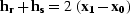 (Figure amosym). The
two-point traveltime function in reflecttt transforms to the form
(Figure amosym). The
two-point traveltime function in reflecttt transforms to the form
|  |
|
| (33) |
Applying the second equation from fermat, we get a simple linear
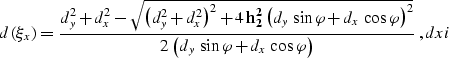
equation for , which has the explicit solution xiy.
From x02xi and xiy one can find the reflection
point location for given midpoint and offset. To find the limits of
possible output midpoint locations, we constrain the reflection
point to be inside the ellipsoid ellips similarly to the way we did
in two dimensions when deriving x0leq. First, let's consider the
case of y2=y1 (the output midpoint is on the line drawn
through in the direction of the input azimuth). In this
case, combining expression xiy and inequality xiyleq
produces
|  |
(34) |
For any azimuth rotation angle  less than 90 degrees, the
limitation x0leq3D is smaller than that of the DMO operator
x0leq. The difference increases with the decrease of the
azimuth rotation, since the AMO aperture section
on the line y2=y1 monotonously shrinks to a point x2=x0=x1
when approaches zero. To extend this conclusion to the whole
3-D aperture, we can find the contour of the aperture by putting the
reflection point
at the edge of the ellipsoid ellips, as follows:
less than 90 degrees, the
limitation x0leq3D is smaller than that of the DMO operator
x0leq. The difference increases with the decrease of the
azimuth rotation, since the AMO aperture section
on the line y2=y1 monotonously shrinks to a point x2=x0=x1
when approaches zero. To extend this conclusion to the whole
3-D aperture, we can find the contour of the aperture by putting the
reflection point
at the edge of the ellipsoid ellips, as follows:
|  |
(35) |
and solving xiy for y2. The aperture contour can then be defined by
the system of parametric expressions
|  |
(36) |
|  |
(37) |
where
|  |
(38) |
 ,and
,and  is defined by edge.
Next: About this document ...
Up: Table of Contents
Stanford Exploration Project
5/9/2001