Short Note
An example of inverse interpolation accelerated by preconditioning

Sean Crawley

sean@sep.stanford.edu

INTRODUCTION

Prediction error filters can be used in a variety of ways to interpolate missing data. One of the main problems with inverse interpolation is its speed. Filters tend to be small, and thus take a long time to propagate information into unknown portions of the much larger model. One answer to this problem is a change of variables, to something closely related to the model but which has the property that information is propagated through it more quickly. Claerbout has demonstrated that a variation on causal integration can be used in the change of variables role, and considerably speed up inverse interpolation on a trace. I apply two-dimensional integration as a preconditioner to the SeaBeam missing data problem in order to decrease the number of iterations required for convergence.

This is one of two papers dealing with nonlinear inverse interpolation applied to the April 18th SeaBeam data set, and methods of speeding up convergence. The other paper, (), is concerned with the use of a multigrid method to this end. More information on the data set and the theory behind inverse interpolation can be found there, as well as in Claerbout's book Three-Dimensional Filtering. In addition, a further occurence of the use of integration as a preconditioner may be found in ().

Here I present an example of integration used as a preconditioner, and echo the positive finding that it can significantly reduce the computational effort of inverse interpolation.

PRECONDITIONING

Given a regression $d \approx Fm$ it is straightforward to formulate an inversion for the model m, given data d and operator F. Instead of m, in some cases it may be computationally easier to solve for some new set of variables x, related to the model by m = Cx. The question is which operator C accomplishes this? One answer is causal integration. A small filter takes many iterations to distribute information through the model; choosing integration as a preconditioner provides a way to distribute information more quickly because it spreads information from one model bin to many. Unfortunately, a simple implementation of causal integration does not yield satisfactory results. Here I use an extension to two dimensions of Claerbout's double symmetric integration.

In this case, the change of variables C actually looks like this:

m = (B'B + BB')x

Where B is a two dimensional leaky integration operator, and B' is its adjoint. With C = B'B + BB', C is self-adjoint: C = C'.

Leaky integration is similar to causal integration. In one dimension, causal integration is equivalent to convolution with a vector of ones:

$$\{ 1,1,\cdots \}$$

By comparison, leaky integration is equivalent to convolution with a vector whose ith element is $\rho ^{i-1}$:

$$\{ 1,\rho ,\rho ^2,\cdots \}$$

The value of $\rho$ is a parameter chosen to be between zero and one.

The inversion is formulated in the same way as is seen in () (refer there or to TDF for a full description of this problem), except that the solver modifies the new variable x at each iteration rather than the model m directly. Three calls to the change of variables are required in each iteration. The gradient direction for the model is computed as before:

$$\Delta m = L'r_d + A'r_m$$

Where m is the model, L the linear interpolation operator that relates data and model space, A a prediction error filter (which is being solved for simultaneously with the model), and r_d and r_m the data and model residuals, respectively. From $\Delta m$, a change in the new variable $\Delta x$ is calculated, and then $\Delta m$ is recalculated:

$$\Delta x = C'\Delta m$$

$$\Delta m = C\Delta x$$

The conjugate gradient solver computes a solution step length for $\Delta x$ and updates the variable x. The third call to the change of variables comes after the solver step to update the model:

m = Cx

An important consideration is the choice of the integration leak factor $\rho$. A low value of rho decreases the degree to which the integration helps speed the inversion along. Information is not propagated as far before it damps away. An excessively high $\rho$ smears the model. The best results in this case were obtained with $\rho =.7$.

Preconditioning and Multigrid incompatibility

This implementation of preconditioning works well where there is no initial guess at the solution, and both the model and x start as zeroes. Unfortunately, without knowing the inverse of C, an initial x₀ for a nontrivial m₀ (initial model not zero) is difficult to find. Because C is an integration, it's a good guess that some differentiation operator will provide something nearly inverse to C, and in this way the preconditioner might be made applicable in cases where there is a good starting guess, for instance in a multigrid inversion. I haven't been successful in formulating an approximation to C^-1 that proves good enough to make a successful combination of multigrid and preconditioning. The utility of such a combination is doubtful; my experience has been that this type of preconditioning only proves helpful where iterations are expensive, and employing the multigrid method tends to make most of the required iterations easy (). In addition, this implementation of preconditioning works by spreading information into large unknown areas. Since the starting models provided by the multigrid method have already been filled with appropriate values, it seems that adding the integration steps would just add computational effort to the problem.

RESULTS

Inverse interpolations with and without the preconditioner were applied to the SeaBeam data, displayed after basic binning in Figure ras18. The results are displayed in Figures levint and prenon.

 

ras18 Figure 1 April 18th SeaBeam data after binning.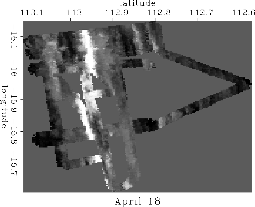

 

levint Figure 2 Nonlinear inverse interpolation by Claerbout after 7,000 iterations.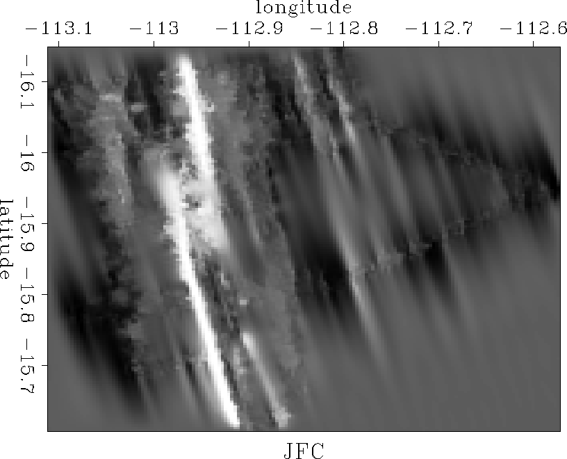

 

prenon Figure 3 Nonlinear inverse interpolation with preconditioning after 2,000 iterations.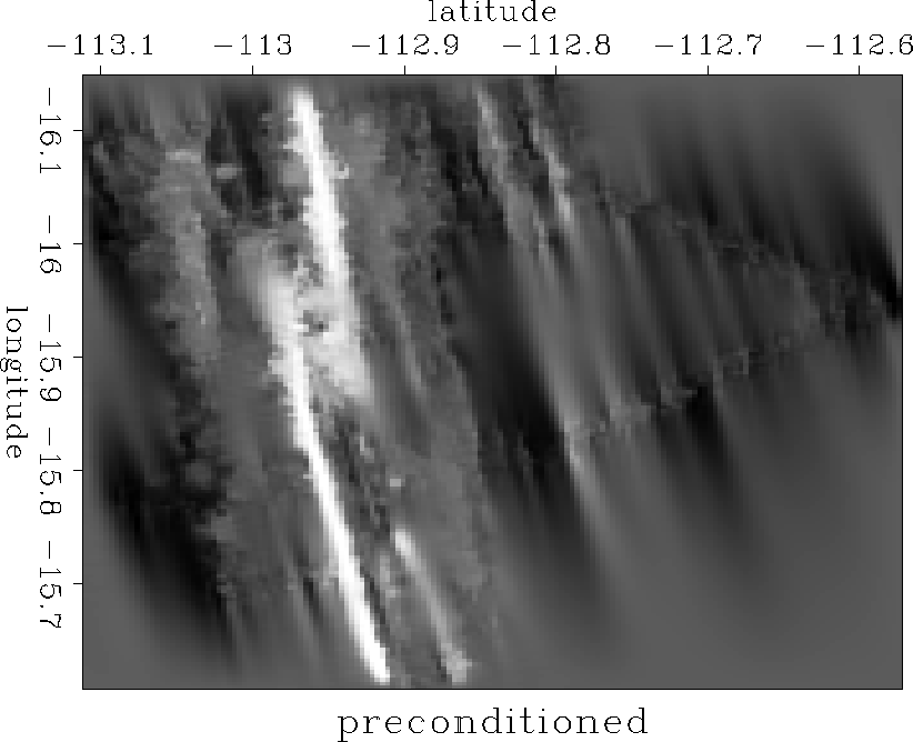

CONCLUSIONS

The two results are essentially identical, as hoped. This indicates that our change of variables is implemented well enough that we do not lose information in adding the extra level of abstraction. The inversion with preconditioning did require considerably less time to run than the inversion without. The standard inversion took over 300 cpu minutes to converge, running on our HP 700. With preconditioning about half that time was required.

[sean,SEP,MISC]