

![[*]](http://sepwww.stanford.edu/latex2html/prev_gr.gif)


ABSTRACTWe present a method for unwrapping the phase of a satellite data set that maps Mt.Vesuvius in Italy. The method finds a solution for a partial differential equation by redefining the problem as a system of regressions that we solve using linear inversion techniques with iterated reweighting. We show three different techniques for eliminating the noise bursts from the raw data and fitting it to a linear model. The first process is a two-step solution in which the data is first cleaned up and then fitted to a model by phase unwrapping. In the second approach, starting from a raw noisy data, we solve the inversion problem as a system of regressions using iterative weighting based on the residual. The third technique attempts to resolve a discontinuity in the data by solving a different system of regressions with weights based on the model. In the three processes, the inversion successfully unwrapped the phase of the radar image and produced an altitude map of the volcano region. We were able to accelerate the convergence of the solution by a smart preconditioning substitution. This transformation changes the problem-formulation variable using a leaky integration operator as a preconditioner. The substitution reduced the number of iterations in the least square-inversion by two orders of magnitude and provided a solution after very few iterations. The method, however, did not help resolve a presumed discontinuity in the model, and we may have to determine an optimal function for the iterated reweighting. |
INTRODUCTION
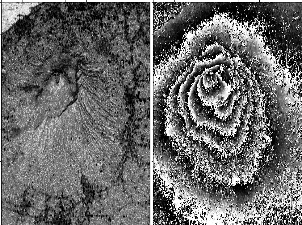
We were presented with
two radar signals, s1(x,y,t) and s2(x,y,t),
from
two satellite orbits 54 meters apart and 800 km above the surface.
The signals were Fourier transformed
and one was multiplied by the complex conjugate of the other, leading to
the power spectrum ![]() ,
whose square root gives
the amplitude function, while the phase can be computed from the
mathematical definition of a complex number.
The straight mathematical definition for the phase function leads to a
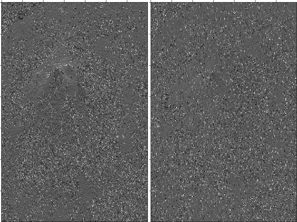
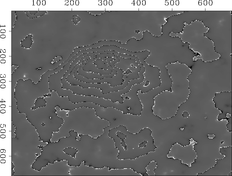
solution of a wrapped phase rather than a true phase. As a result, when
looking at the phase map in Figure original, we do not see
a hill-like structure, but rather
something resembling a contour map.
The contours of constant phase appear to be contours of constant altitude,
which leads us to suppose that a study of radar theory would lead to a linear
relation between phase and altitude. Actually, the altitude would be measured
along the viewing angle, which happens to be 23 degrees from the vertical.
The viewing angle is such that the mountain blocks some of the
landscape behind it. Therefore, in that region, the contour lines
join together,
suggesting a jump in the altitude function over the hidden terrain.
,
whose square root gives
the amplitude function, while the phase can be computed from the
mathematical definition of a complex number.
The straight mathematical definition for the phase function leads to a
solution of a wrapped phase rather than a true phase. As a result, when
looking at the phase map in Figure original, we do not see
a hill-like structure, but rather
something resembling a contour map.
The contours of constant phase appear to be contours of constant altitude,
which leads us to suppose that a study of radar theory would lead to a linear
relation between phase and altitude. Actually, the altitude would be measured
along the viewing angle, which happens to be 23 degrees from the vertical.
The viewing angle is such that the mountain blocks some of the
landscape behind it. Therefore, in that region, the contour lines
join together,
suggesting a jump in the altitude function over the hidden terrain.
The problem of uncovering the true phase from the complex data is known as phase unwrapping, for which we present a solution based on Claerbout's derivations. The solution reformulates the problem as a system of regressions that can be solved using linear least-square inversion techniques. We use iterated reweighting to estimate weighting functions based on the residuals or on the updated model of the previous iteration. Weighting with residual-based functions is a method of despiking that handles noise bursts in the residual. Similarly, model-based weighting functions handle noise bursts in data from a model that changes rapidly because it is high frequency or has jumps of discontinuity; such is the case with our altitude function.
For such a two-dimensional problem, convergence speed represents some problems. Our model contains 700 by 700 mesh points; so, theoretically, convergence is achieved after about half a million iterations. Even though in practice we only use a few thousand iterations, the convergence is still considerably slow. One way to accelerate the convergence is to make a change of variables and recast the problem in terms of an intermediate quantity. In a second stage we evaluate the solution for the original problem as a function of the intermediate solution.
In the next sections we will show how we estimate the weighting functions in the regressions and how we chose the preconditioning operator, but first we start by defining the phase unwrapping problem.
 |


PHASE UNWRAPPING
A complex number is defined as:
 |
(1) | |
| (2) | ||
| (3) |
 |
(4) | |
| (5) | ||
| (6) |
 |
(7) | |
| (8) | ||
| (9) | ||
| (10) |
| (11) |
| (12) |
 |
(13) |
| (14) |
MODEL FITTING
Given very noisy raw data, our biggest challenge was handling the noise spikes and bursts while attempting the phase unwrapping. We used three different techniques to clean up the data and unwrap its phase:
De-bursting with Iterated reweighting
A method for creating cleaned up data ![]() from the noisy data phase gradient
from the noisy data phase gradient ![]() is solving the regression
is solving the regression
| (15) | ||
| (16) |
Roughly, we want a weight wi=|ri|-1/2 for medians and wi=|ri|-1 for modes. To avoid zero division and to handle small values in the usual L2 way we use weights such as those used in Claerbout :
 |
(17) | |
| (18) |
| (19) |
Once the data phase gradient has been filtered
using regressions (15) and (16), the
problem is reduced to performing the phase unwrapping by the solution of
![]() .
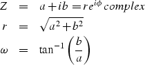
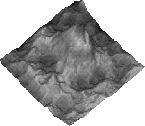
Figure method1 shows the results of the inversion. An altitude map
of the mountain is uncovered and outlines the shape of the volcano.
.
Figure method1 shows the results of the inversion. An altitude map
of the mountain is uncovered and outlines the shape of the volcano.
Fitting noisy data to a linear model
In this approach, we fit the noisy data phase gradient ![]() to a linear model, say
to a linear model, say
![]() ,using the following regressions:
,using the following regressions:
| (20) | ||
| (21) |
We needed to experiment with the free parameter ![]() in mtd2.
A good result was obtained for
in mtd2.
A good result was obtained for ![]() .Notice that this approach is very similar to the first method
of cleaning up the data phase gradient and then applying the
phase unwrapping solution. The two operations are here combined
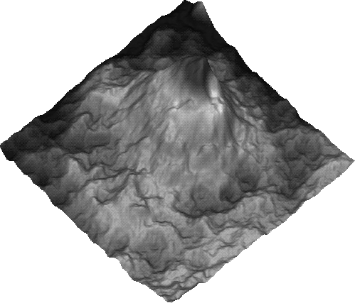
in a single system of regressions. Figure method2 shows the results of the
inversion. The method succeeded in uncovering the hill shape of the volcano.
.Notice that this approach is very similar to the first method
of cleaning up the data phase gradient and then applying the
phase unwrapping solution. The two operations are here combined
in a single system of regressions. Figure method2 shows the results of the
inversion. The method succeeded in uncovering the hill shape of the volcano.
 |
 |
 |
 |
Fitting noisy data to a discontinuous model
The previous approach handled noise bursts in the residual, which is not the same as noise bursts in the data. We then attempted to fit the data phase gradient to a model with discontinuity jumps using the following regression:
| (22) | ||
| (23) |
 |
(24) |
| (25) |
 |
PRECONDITIONING BY INTEGRATION
Convergence speed was something of a problem in this data set; about 2000
iterations were required to achieve a solution for the phase map.
Resampling to every other mesh point, although reduced the computational
time, did not actually decrease the number of iterations.
Later we used a change of variables to accelerate the iterative inversion. The
preconditioning substitution changes the problem formulation variable ![]() in inverse to a new variable
in inverse to a new variable ![]() . We used a leaky
integration operator () as a preconditioner so that
the new variable
. We used a leaky
integration operator () as a preconditioner so that
the new variable ![]() is like the derivative of the solution phase
is like the derivative of the solution phase ![]() .By the preconditioning transformation
.By the preconditioning transformation ![]() ,
we have recast the original
inversion relation inverse into
,
we have recast the original
inversion relation inverse into
| (26) |
DISCUSSION
Each of the procedures discussed above has yielded a final phase function that describes an altitude map of a volcano. Methods (1) and (2) are quite similar with the exception of data cleaning and model fitting being done in two stages in (1) by solving the regressions:
| (27) | ||
| (28) |
| (29) |
| (30) | ||
| (31) |
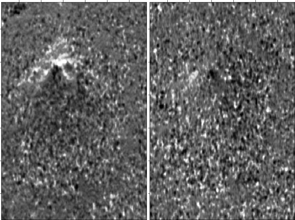
To better illustrate the altitude map around the hidden terrain
behind the mountain,
we plotted the function ![]() . The plot should
look similar to that of the initial phase map.
The frequency factor, a,
controls the number of contours used in the display.
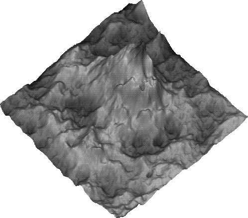
Figure display-grad-bw shows a contour map
of the results of method 3. As we notice, the
contours are more continuous than in the original phase map. The
technique, however, did not resolve the presumed discontinuity in
the hidden section of the mountain. Although the contours come very close
together around that region, they do not actually join,
but rather remained parallel.
. The plot should
look similar to that of the initial phase map.
The frequency factor, a,
controls the number of contours used in the display.
Figure display-grad-bw shows a contour map
of the results of method 3. As we notice, the
contours are more continuous than in the original phase map. The
technique, however, did not resolve the presumed discontinuity in
the hidden section of the mountain. Although the contours come very close
together around that region, they do not actually join,
but rather remained parallel.
The inability to image the discontinuity illustrates that there is a significant room for improvement. In order to understand why the discontinuity was not imaged and to come up with a scheme that is capable of solving for the jump in the altitude map, we need to test our technique on a synthetic model that simulates the nature of the discontinuity in the Vesuvius data set. To obtain the correct altitude map we must migrate the data around the fault instead of straight integration across it. Future goals of this effort will target testing the method on canonical models and optimizing the weighting functions used in the iterated reweighting.
 |
CONCLUSIONS
We have presented a technique for unwrapping the phase of a radar image of Mt. Vesuvius in Italy. The method finds a solution for a partial differential equation by redefining the problem as a system of regressions that we solve using iterative linear inversion techniques. The biggest challenge was handling the noise spikes and bursts in the raw data set. Three different techniques were used for cleaning up the data and fitting it to a model. The techniques use iterated reweighting by functions that are based on the residual or the model. The results of the inversion were quite accurate in uncovering the hill shape of the volcano. The convergence of the solution was accelerated by a change of variable using a leaky integration operator as a preconditioner. This substitution reduced the number of iterations by two orders of magnitude and provided a very rapid solution. The method, however, did not resolve for the presence of a discontinuity in the altitude map. We suspect that the sharpness of the image will be improved with the use of optimal functions in the iterated reweighting.
ACKNOWLEDGEMENTS We thank Umberto Spagnolini of Politecnico di Milano for providing us with the data. He recently submitted a paper on the subject to IEEE Trans. Geoscience and Remote Sensing.
[MISC,paper]