The interpolation of a 3-D data set by a pair of 2-D filters

Matthias Schwab and Jon F. Claerbout

matt@sep.stanford.edu, jon@sep.stanford.edu

ABSTRACT

Seismic 3-D field data is often recorded as a set of relatively sparse and often irregular 2-D lines. Under the assumption that the data consists of the superposition of local plane waves, such data can be interpolated by prediction-error techniques using a set of two 2-D filters instead of the conventional single 3-D filter. The two 2-D prediction-error filters are found by two independent linear minimization problems along sets of parallel linearly-independent lines. A third linear minimization yields the missing data. Fortunately, such an approach avoids the nonlinear minimization that is required when trying to find simultaneously the missing data and the 3-D filter on a sparse 3-D data set.

INTRODUCTION

Interpolation of data arises whenever shortcomings in the recording geometry result in irregular, aliased, or even missing data. Claerbout discusses methods of interpolating data by data-adaptive prediction-error filters (PEF). A PEF interpolation algorithm computes the coefficients of the prediction-error filter and the missing data. If the data contains a sufficiently large, continuous patch of known data, then the filter can be found before the missing data is estimated. The data interpolation amounts to a two-stage linear optimization. If the known data does not contain such a sufficiently large continuous patch, than the filter and the missing data are estimated simultaneously by a nonlinear optimization process. The two-stage linear approach converges reliably and is therefore preferred over the nonlinear approach.

In this paper I claim that for the interpolation of 3-D data, which consists of superposed plane waves, a set of two 2-D prediction-error filters suffices. Usually, a 3-D interpolation filter is used to interpolate 3-D data. Interpolation using a single 2-D interpolation filter neglects all information along the third dimension and yields, in general, an inferior, interpolated image. I suggest, however, in this paper that a combination of two 2-D filters captures the full three dimensional information of a data set consisting of a superposition of plane waves. Claerbout proposes a similar approach for the annihilation of coherent events.

Why would anyone prefer interpolation by a pair of 2-D filters over interpolation by a single 3-D filter? Seismic data is often collected along lines. These lines are 2-D data planes in a seismic data cube, such as a shot-gather. Such a data plane is a data patch that permits the estimation of a 2-D prediction-error filter by linear optimization even when the sparseness of such lines requires a nonlinear approach for a standard 3-D filter. The method is, for example, applicable when merging overlapping 3-D surveys.

THEORY AND 1-D SYNTHETIC EXAMPLE

The test data set shown in Figure duelin is a superposition of three functions that I call plane waves. One plane wave looks like low-frequency horizontal layers. The various layers vary in strength with depth. The second wave is dipping about $45^\circ$ down to the right and its waveform is perfectly sinusoidal. The third wave dips down to the left and its waveform is bandpassed random noise as in the horizontal beds. These waves will be handled differently by different processing schemes. To identify them clearly it may be halpful to view the figure at a grazing angle from various directions.

 

duelin
Figure 1 Synthetic wavefield (left) and as observed over survey lines (right).

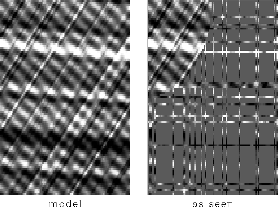Obviously we can fill in between lines by minimizing the power out of a Laplacian operator but it is better to minimize the power out of a prediction-error filter (PEF). In practice, the problem is, where do we get the PEF? Figure duelin shows an example of sparse tracks except that it is not realistic (I will use it for calibration) in the upper left corner where in a quarter circular disk the data covers the model densely. Such a dense region is ideal for determining the PEF. Indeed, the two-stage linear interpolation by a 2-D filter cannot determine a 2-D PEF from the sparse data lines because any place you put the filter (unless there are enough adjacent data lines) it will multiply missing data so every regression equation is nonlinear and abandoned.

Before we use the dense data region and before we leap to the nonlinear regression, there are a few tricks that get us started towards the desired result. (When we do try a nonlinear approach it is helpful and often essential to have a good starting guess.) The idea is simply this: if it is too hard to estimate a 2-D PEF, we instead estimate a 1-D PEF, or better yet, we estimate a 1-D PEF for east-west tracks and a second 1-D PEF for north-south tracks. Let $\bold A$ be the east-west PE operator and $\bold B$ be the north-south operator and let the signal or image be $\bold h = h(x,y)$.The regressions we pose are

$$\begin{eqnarray} \bold 0 &\approx& \bold T \bold h - \bold d \\ \bold 0 &\approx... ...d h \\ \bold 0 &\approx& \bold B \bold h \EQNLABEL{maskregression}\end{eqnarray}$$ (1) (2) (3)

where $\bold d$ is the data and $\bold T$ is a point-to-point mapping that I often call the tracking operator. This operator copies values from the desired image space $\bold h = h(x,y)$to the data space. The data space could be organized in a variety of ways. For theoretical examples it is easiest to let the data space be a grid that overlies the image space. At each location the tracking operator multiplies the image by either a one or a zero depending on whether data is recorded at that location. This operator is often called a mask and can be thought of as an identity matrix with some of its ones missing. In practice, the data space is generally organized as tracks.

 

duelversus
Figure 2 Data infilled by two 1-D PEFs (left) and by one 2-D PEF (right).

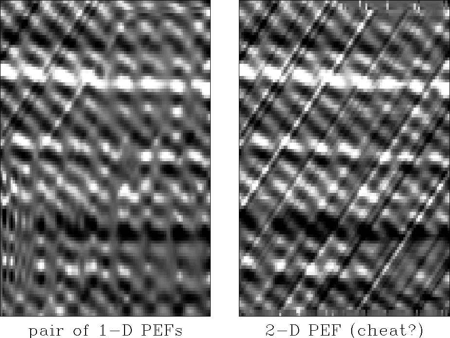To get the 2-D PEF, I used the two-stage linear interpolation scheme and I was dependent on the cheating corner of dense data. The purpose for cheating here is to establish motivation for the more difficult task of doing the nonlinear estimation on data lines, where cheating would be impossible. Figure duelversus compares the use of two 1-D PEFs versus a single 2-D PEF. Studying Figure duelversus, we observe that in correspondence with prediction-error theory:

• Predictable with two 1-D filters:
  • Horizontal (or vertical) plane wave with random waveform
  • Dipping plane wave with a sinusoidal waveform
• Predictable with one 2-D filter:
  • both of the above
  • Dipping plane wave with a random waveform

3-D FIELD DATA EXAMPLE

Having demonstrated for a synthetic data case that a set of 1-D filters suffices in interpolating certain types of 2-D data, this section is going to extend the extension of this concept to the interpolation of a 3-D field data example.

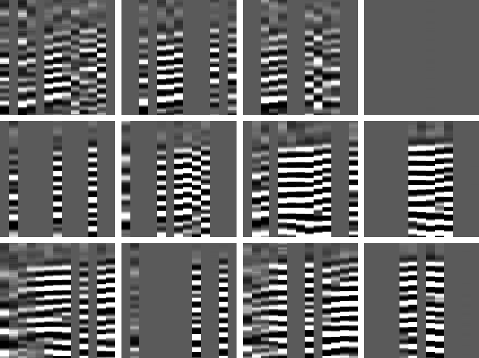
Several years ago the Stanford Exploration Project collected seismic data in an experiment in the hills west of Stanford(). The geophone groups were organized out in a quadratic mesh of 13 by 13 nodes. The data cube selected for the interpolation comprises 150 time samples. The original data is displayed as 12 slices of 13 traces in Figure orig. About half of the traces of the recorded data contain no values because of instrument failure.

 

orig
Figure 3 Original data before interpolation. The original data is a 13 by 13 grid of traces which shows the arrival of a quarry blast event. Many of the traces are dead.

The data geometry allows a two-stage linear interpolation approach using a 3-D prediction-error filter. The filter's extension in the (x,y)-dimensions is restricted by the size of a continuous, known data patch. The filter of the shape

        a1=5 a2=3 a3=2   lag1=3 lag2=2 lag3=1

yields the interpolated data displayed in Figure miss3d. The blank data slice in the left-hand corner of the original data is filled in by interpolation of neighboring data slices. Some traces are not interpolated and I assume that the neighboring traces are inconsistent with the overall data spectrum. However, the prediction-error interpolation yields data that continues the dip of the original field data and decreases smoothly in amplitude as the interpolation distance increases. The interpolation succeeds in the sense that the interpolated data is hardly distinguishable from the original data. In the following discussions I will use the interpolated data of this 3-D interpolation approach as a reference for evaluating the success of the subsequent interpolation schemes.

 

miss3d
Figure 4 Data interpolated by 3-D filter.

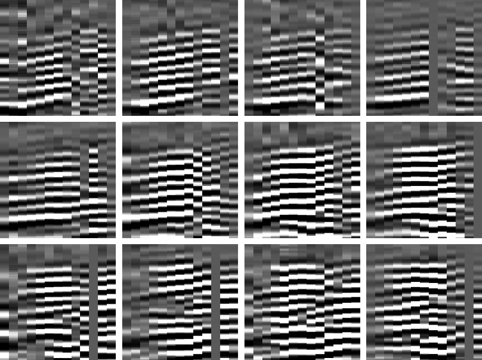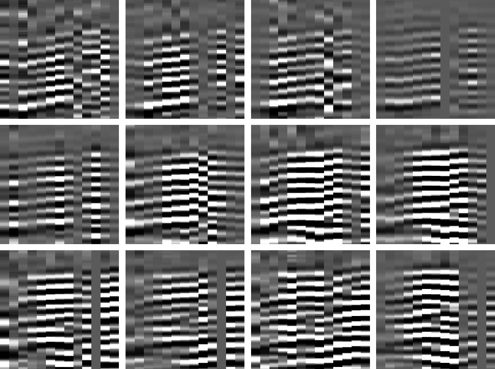
In Figure missxy the data is interpolated given following two 2-D filter shapes:

        a1=5 a2=3 a3=1   lag1=3 lag2=2 lag3=1  
        b1=5 b2=1 b3=2   lbg1=3 lbg2=1 lbg3=1

The two filters lie in the (x,z) and (y,z) data planes. The data interpolation is of similar quality to the one in Figure miss3d. Close examination shows that the amplitude of the interpolated data decreases faster with interpolation distance, than it is the case in the reference 3-D scheme.

 

missxy
Figure 5 Data interpolated by two 2-D filters in (x,z) and (y,z) planes.

Interpolation by a set of filters in the (x,z) and (x,y) planes yield Figure missxz. The shapes of the filters are:

        a1=5 a2=3 a3=1   lag1=3 lag2=2 lag3=1
        c1=1 c2=3 c3=2   lcg1=1 lcg2=2 lcg3=1

Again, the prediction-error interpolation results in a data cube comparable with the reference one in Figure miss3d. The rate of energy loss with interpolation distance is comparable with the previous scheme using two vertical 2-D filters. In the author's experience, the horizontal filter in the (x,y) plane tends to increase the rate of convergence when interpolating the almost horizontal event.

 

missxz
Figure 6 Data interpolated by two 2-D filter in (x,z) and (x,y) planes.

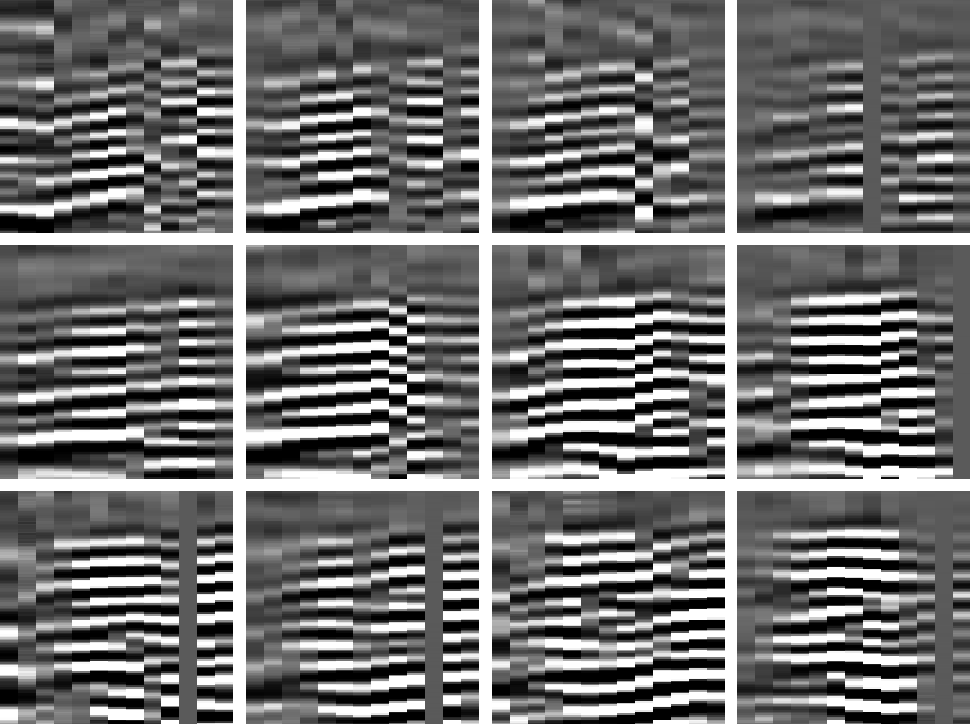Figure diff compares the sixth data slice of the previous interpolations. The top-right panel shows the data slice interpolated by two filters in the (x,z) and (y,z) planes. The right top panel shows the difference between the data slice to its left and the corresponding slice of the reference interpolation using a 3-D filter (Figure miss3d). The lower panel pair shows the same data slice interpolated by two filters in the (x,z) and (x,y) planes and the difference with respect to the reference data slice. There is significant energy remaining in the difference plots. The energy shows coherent linear trends which are consistent with the dip of the data.

 

diff Figure 7 Difference plots for sixth data slice. The top row is the data interpolated by filters in the (x,z) and (y,z) planes. The bottom row is the data interpolated by filters in the (x,z) and (x,y) planes. The left column displays the difference of the interpolated data to the right with the reference data computed using a 3-D filter.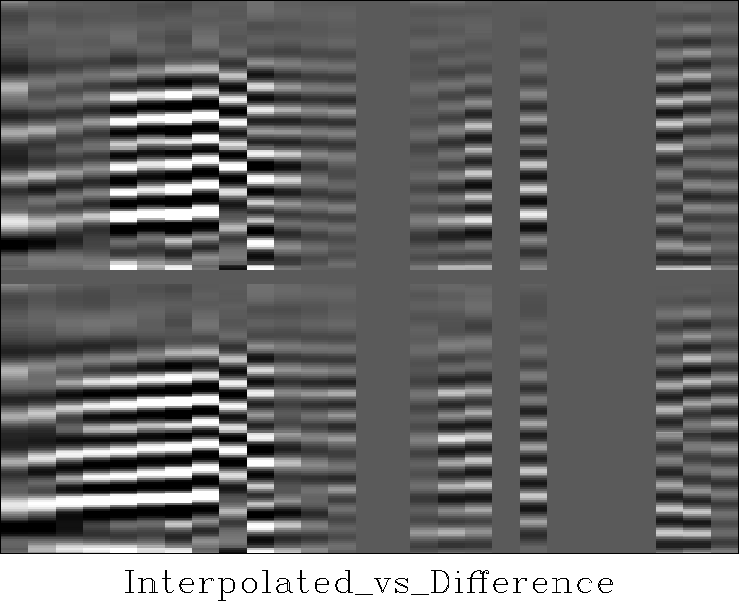

Various other combinations of 2-D and 1-D prediction-error filters, such as a set of three 2-D filters in the (x,z),(y,z), and (x,y) planes, yielded comparable results to the two 2-D filter interpolation presented here.

CONCLUSIONS

In general the interpolation of certain n-dimensional data can be accomplished by a set of (n-1)-dimensional prediction-error filters. In the 2-D case, the data which is predictable (and therefore interpolated correctly) comprises horizontal events of arbitrary waveform and dipping events of sinusoidal waveform. In the 3-D case, the data which is predictable includes dipping plane waves of random waveform.

Considering a recording geometry that is continuous and dense along a sparse set of 2-D slices of a 3-D data cube, the 3-D interpolation of wavefields can be accomplished by a two-stage linear prediction-error approach. This technique allows the application of reliably converging linear inversion techniques to data sets that seem to require nonlinear interpolation. As shown in a synthetic 2-D analogue case and in a 3-D field data case, the quality of the interpolated data is roughly comparable to the quality of the standard interpolation by a single 3-D filter. In the author's experience, the computational effort for interpolation by two 2-D filters is slightly higher than the one by a single 3-D filter, when both techniques are applicable.

I conclude that if possible the prediction-error filter interpolation involving a full 3-D filter is preferable over interpolation involving a set of 2-D filters. If the sparseness of the original data prevents the application of such a 3-D two-stage linear approach, the linear two-stage approach involving a set of 2-D filters offers a valuable alternative to a nonlinear interpolation method.

[MISC,SEP]