Compensating for irregular sampling and rugged topography

Dimitri Bevc

dimitri@sep.stanford.edu

ABSTRACT

Artifacts arise when irregularly sampled data are input to a Kirchhoff datuming algorithm. The irregular sampling occurs because of uneven sampling of the recording surface and rugged topography. To ameliorate these artifacts, I combine wave-equation datuming with model-space filtering to resample data onto a regular grid. The filtering can be a simple Laplacian operator or a nonstationary prediction error filter with unknown filter coefficients. Synthetic examples demonstrate that the method is successful for unevenly sampled data along a flat datum. The best result is achieved by using a Laplacian filter in the inversion.

Kirchhoff wave-equation datuming can be used to regularize unevenly sampled data (Zhang and Claerbout, 1992). Although the kinematics are correctly restored, artifacts arise from the irregular sampling of the input data. These same artifacts arise when the data are sampled evenly in areas where rugged topography has severe discontinuities (Bevc, 1992). In the presence of both irregular sampling and rugged topography, the problem is compounded. To overcome these difficulties, I formulate wave-equation resampling as an inverse problem which transforms the data from an irregularly sampled rugged datum to a regularly sampled flat datum.

In this report I describe the theory of inverse datuming and apply it to synthetic data. I resample the data using just the datuming operator, and with inversions of varying complexity. In the most complex example, I implement the inversion so that I simultaneously solve for the output data and the nonstationary prediction error filter (PEF) which estimates the inverse covariance (Claerbout, 1994). Further work is required to determine the best parameters to use in the most sophisticated inversion, but so far the best results are attained by using a Laplacian operator as an estimate of inverse covariance.

THEORY

The concept of wavefield resampling by upward continuation is illustrated in Figure ksample. Application of the Kirchhoff upward continuation operator ${\bf K}^{ \dag }$ transforms the irregularly sampled data ${\bf d}$ from the rugged topography to the regularly sampled data ${\bf m}$ along a flat datum. The detailed form of the Kirchhoff operator and its adjoint has been described in previous reports (Bevc, 1994).

 

ksample Figure 1 Upward continuation from an irregularly sampled rugged topography to an evenly sampled flat datum. Input traces d are time shifted, weighted, and summed into output locations m.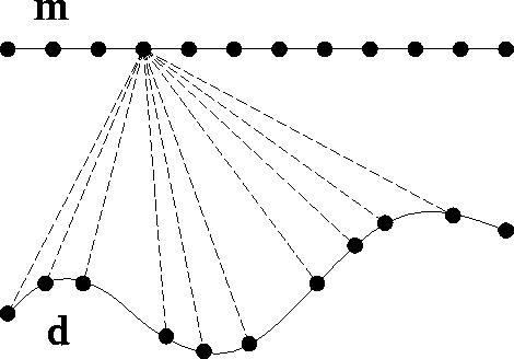

The inverse problem is formulated by writing down the regression:

$$\EQNLABEL{regression} \begin{array} {ccl} {\bf 0} & \approx & {\bf d - K m} \\ {\bf 0} & \approx & {\bf A m},\end{array}$$ (1)

where ${\bf d}$ is the irregularly sampled data, ${\bf K}$ is the Kirchhoff downward continuation operator (adjoint of upward continuation), and ${\bf m}$ is the regularly sampled output that we are solving for. ${\bf A}$ is the inverse covariance matrix.

If the inverse covariance matrix is unknown (as is usually the case), it can be estimated by considering ${\bf A}$ to be a prediction error filter with coefficients to be determined (Claerbout, 1994). The model and the prediction error filter can then be written as

$$\EQNLABEL{bothunk} \begin{array} {ccl} {\bf m} & = & {\bf m... ... m} \\ {\bf A} & = & {\bf A}_i + {\bf \triangle A},\end{array}$$ (2)

where the subscript i indicates initial values which are to be updated. The product of the filter and the model is

$$\EQNLABEL{nlproduct} \begin{array} {ccl} {\bf Am} & = & ({\b... ...bf \triangle A m}_i + {\bf \triangle A \triangle m}.\end{array}$$ (3)

The regression equation regression then becomes:

$$\EQNLABEL{nlregression} \begin{array} {ccl} {\bf 0} & \appro... ...bf \triangle A m}_i + {\bf \triangle A \triangle m}.\end{array}$$ (4)

Dropping the nonlinear term and rearranging, the final regression can be written as:

$$\EQNLABEL{peftomoreg} \begin{array} {ccl} {\bf d - K m}_i & ... ...pprox & {\bf A}_i{\bf \triangle m +\triangle A m}_i.\end{array}$$ (5)

The data space and model space residuals are defined as:

$$\EQNLABEL{residuals} \begin{array} {ccl} {\bf r}_d &\; =\; &... ...- K m}_i\\ {\bf r}_m &\; =\; & {\bf -A}_i {\bf m}_i.\end{array}$$ (6)

Packing the unknown filter coefficients, ${\bf \triangle A}$ into the abstract vector ${\bf \triangle a}$ and putting the elements of the slowness model ${\bf m}_i$ into a convolutional matrix ${\bf M}$,the last convolution of equation peftomoreg can be expressed as ${\bf M \triangle a}$.The regression of equation peftomoreg can then be written in matrix form as

$$\EQNLABEL{pefregression} \left[ \begin{array} {c} {\bf r}_d ... ... {c} {\bf \triangle m} \\ {\bf \triangle a} \end{array}\right].$$ (7)

This system of equations is solved using the method of conjugate gradients. The first step in the solution is to initialize the model by calculating

$$\EQNLABEL{init1} {\bf m}_i \;=\; {\bf K}^{ \dag }{\bf d},$$ (8)

and making an initial guess of the filter

$$\EQNLABEL{laplacian} {\bf A}_i = \partial^2_x + \partial^2_t.$$ (9)

The regression equation pefregression can then be used to calculate the gradient:

$$\EQNLABEL{gradient} \left[ \begin{array} {c} {\bf \triangle ... ...ft[ \begin{array} {c} {\bf r}_d \\ {\bf r}_m\end{array}\right],$$ (10)

and the conjugate gradient:

$$\EQNLABEL{conjgradient} \left[ \begin{array} {c} {\bf \trian... ... {c} {\bf \triangle m} \\ {\bf \triangle a} \end{array}\right].$$ (11)

In summary, the conjugate gradient solution begins by initializing the model and filter with equations init1 and laplacian. The residuals are initialized using equation residuals and iterations begin by calculating the gradient [equation gradient] and the conjugate gradient [equation conjgradient].

SYNTHETIC EXAMPLE

The algorithm is demonstrated on a synthetic shot gather along a planar datum. A Kirchhoff code was used to generate the gather on a coarse grid, which was then subsampled unevenly, so that the sampling interval varies between about 50 m and 150 m (Figure xintsyn). The effect of the irregular sampling is similar to the effect of statics since each trace has a slight departure from hyperbolic traveltime due to the variation in offset (Figure irrsyn).

 

xintsyn Figure 2 Irregular sampling interval of the synthetic data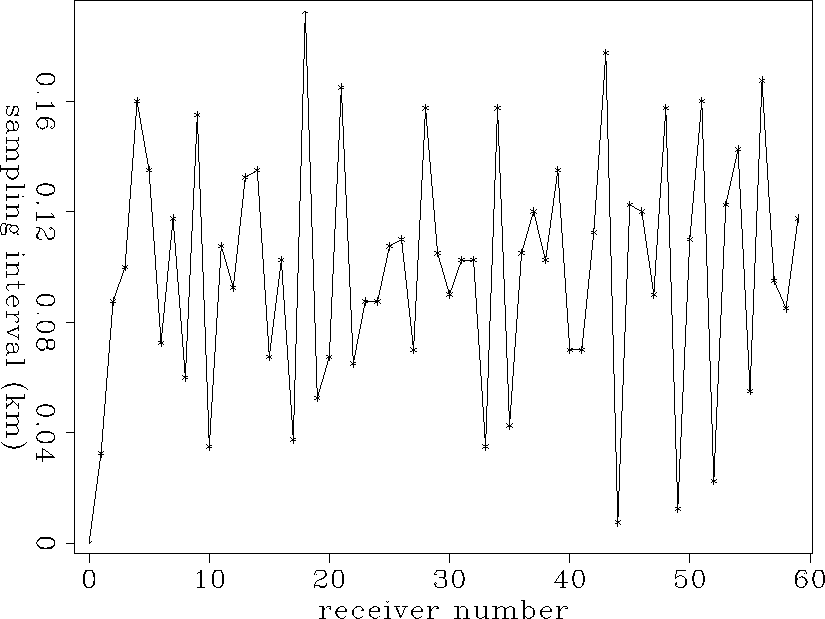

 

irrsyn Figure 3 Irregularly sampled synthetic shot gather. The effect of the irregular sample interval is the step-like moveout seen at far offsets.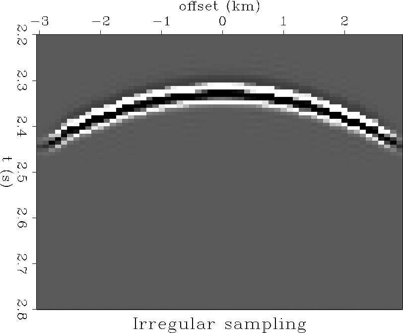

Resampling by redatuming

In Figure wedresamp the synthetic is resampled by upward continuing the data to a regularly sampled datum. This application of the operator ${\bf K}^{ \dag }$ restores the kinematics, but results in the undesirable artifacts which look like diffractions following the hyperbolic event. These artifacts arise because the uneven sampling does not allow the Kirchhoff summation to properly cancel in regions where there should be destructive interference. These streaks are intrinsic to the Kirchhoff operator.

 

wedresamp Figure 4 Wave-equation resampled synthetic. The data of Figure irrsyn have been upward continued to a regularly sampled output datum.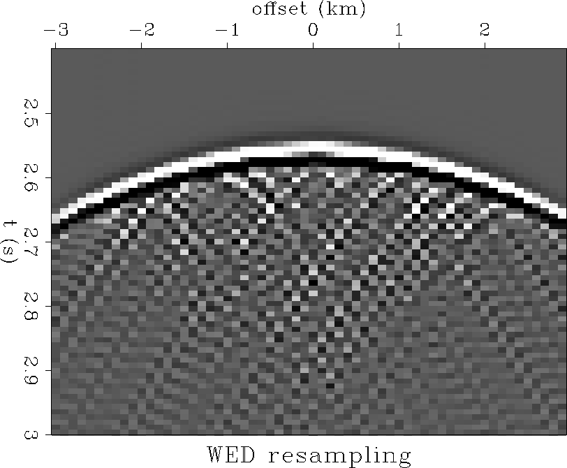

Resampling by inverse redatuming

The first examples of resampling by inverse datuming are performed using equation regression. Using only the top part of the regression, ${\bf 0 \approx d - K m}$ (i.e. no estimate of inverse covariance), results in Figure cgup.40a. We see that performing a conjugate gradient wavefield inversion alone does not eliminate the artifacts because they are required to reconstruct the original data. All of the inversions in this section are the result of 40 iterations of conjugate gradient.

In Figure cgup.40b the inverse covariance is estimated by using a Laplacian operator for ${\bf A}$ in equation regression. This results in an improved resampled output. The undesirable artifacts have been substantially suppressed.

 

cgup.40
Figure 5 (a) Conjugate gradient datuming without any estimate of inverse covariance, and (b) using a Laplacian filter as an estimate of inverse covariance.

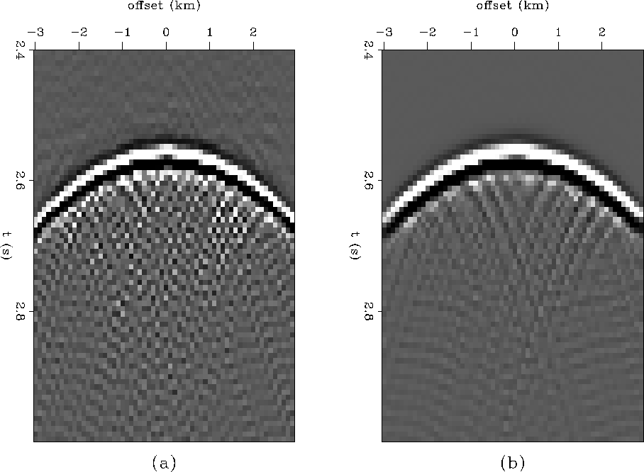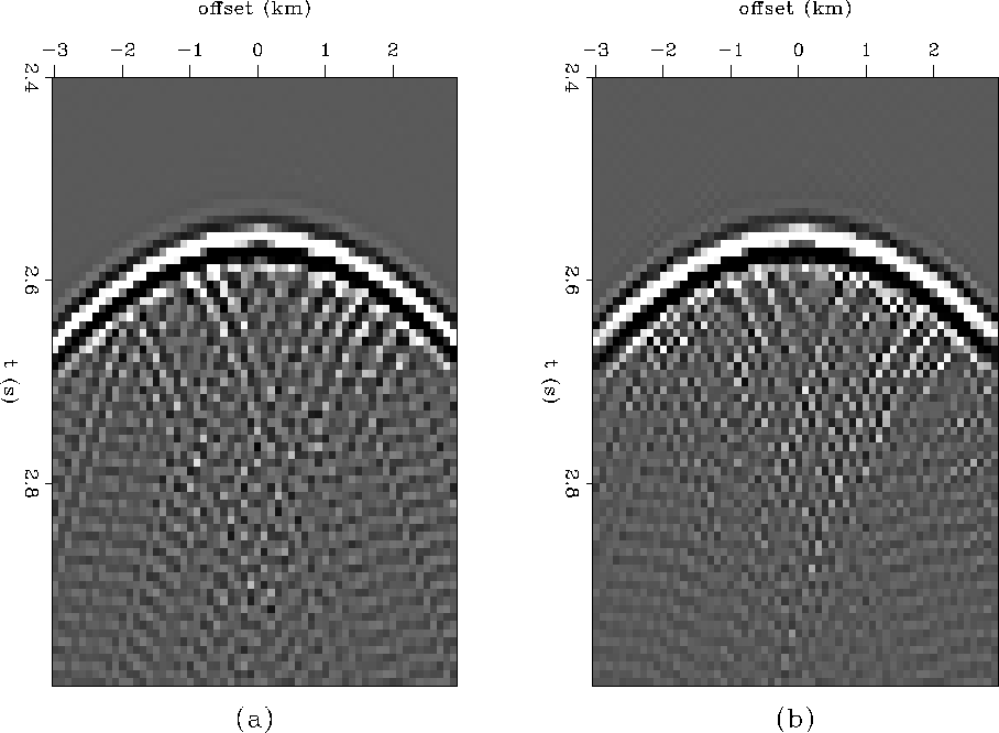
Figure cgresamp.40 is generated by solving equation peftomoreg as outlined by equation init1 through equation conjgradient. In the Figure cgresamp.40a one filter was calculated for the whole data panel. The inversion was run for 20 iterations using the Laplacian filter, and then for 20 more iterations solving simultaneously for the output and the unknown PEF coefficients. The PEF was constrained to be a 3 by 3 filter. Nonstationarity was taken into account in Figure cgresamp.40b by solving for the PEF in 3 overlapping windows. This result is only marginally better than Figure cgresamp.40a.

 

cgresamp.40
Figure 6 (a) Conjugate gradient datuming using a PEF calculated for the whole data panel to estimate inverse covariance, and (b) accounting for nonstationarity by calculating the PEF in patches.

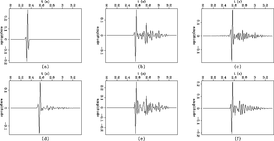
The center traces of the synthetic examples are plotted in Figure amps. The wave-equation resampled and conjugate gradient resampled events (Figure ampsbc) have noisier tails than the results of inverting with the Laplacian inverse covariance estimate (Figure ampsd). As concluded earlier, the best result is obtained using the Laplacian (Figure ampsd). This result has the lowest amplitude tail.

 

amps
Figure 7 Center trace of: (a) original synthetic (Figure irrsyn), (b) wave-equation resampled synthetic (Figurewedresamp), (c) conjugate gradient datuming (Figurecgup.40a), (d) conjugate gradient datuming with Laplacian filter (Figurecgup.40b), (e) conjugate gradient datuming with PEF filter (Figurecgresamp.40a), (f) conjugate gradient datuming with PEF nonstationary filter (Figurecgresamp.40b).

DISCUSSION AND CONCLUSIONS

Further work is required to gain experience in choosing filter coefficients and windows to get optimal inversion results. Shape as well as size and gap of the PEFs has an effect on the inversion result. Using purely lateral prediction filters with zeros on either side of the 1 should be examined. The examples shown here represent a very limited number of possibilities.

The best inversion result for the synthetic data is obtained by using the Laplacian. The nonstationary inversion may not be working well because the windows may have to be larger so that the unknown filter coefficients can be better determined. It is clear that using an additional regression equation to estimate inverse covariance results in a better inversion; however, it is still unclear what kind of filter should be used. Given the added expense and complexity of conjugate gradient datuming with the PEF, it may be better to just use the Kirchhoff operator itself in situations where the topography and irregular sampling are not too severe.

The ultimate goal of this work should incorporate not only resampling, but interpolation of output traces so that there are more output traces than input traces and so that gaps in recording are filled. This will be especially useful for land data in rugged terrain where there are often many more receiver locations than shot locations. The sparse shots tend to be more randomly placed than the receivers.

REFERENCES

• Bevc, D., 1994, Matrix formulation of adjoint Kirchhoff datuming: SEP-80, 373-380.

• Bevc, D., 1992, Kirchhoff datuming with irregular acquisition topography: SEP-75, 137-156.

• Claerbout, J. F., 1994, Applications of three dimensional filtering: preprint in SEP-82.

• Zhang, L. and Claerbout, J. F., 1992, Wave-equation resampling of unevenly spaced traces: SEP-75, 243-249.