Velocity structure of the methane hydrate formation at the Blake Outer Ridge

Christine Ecker

christin@sep.stanford.edu

ABSTRACT

Seismic analysis of data from the Blake Outer Ridge indicates the presence of hydrate-bearing sediments overlaying gas-saturated sediments in this region. In an attempt to determine possible lateral and vertical variations of the hydrate and gas sediments, I performed a 2-D velocity analysis along two approximately perpendicular seismic lines. Subsequent determination of the seafloor and BSR reflection coefficients along one of the lines resulted in additional zero offset P-wave velocity and density constraints. Combining these with the average interval velocity model of this line, I performed a 1-D elastic amplitude modeling of zero offset reflections using the Thompson-Haskell reflectivity method. The results suggest that regions showing a continuous bottom simulating reflection are characterized by a thick hydrate layer that has an average velocity of 2.1 km/s overlaying low-velocity ($\approx$ 1.6 km/s) sediments of considerable thickness. This result agrees well with results discussed in SEP80. In regions of discontinuous BSR, a less pronounced velocity contrast is visible, probably indicating a decrease in the hydrate concentration of the sediments.

INTRODUCTION

Methane hydrate structures are increasingly recognized as being a potential future energy resource and as having a possible strong ``greenhouse'' effect on future global climate (). Recent estimates showed that the amount of hydrocarbons present in hydrate structures is at least twice the amount of recoverable and non-recoverable fuels, such as oil and natural gas. Associated with the pressure-temperature dependent base of the hydrate stability zone are so-called bottom simulating reflectors (BSR). Depending on the origin of the methane necessary to form hydrate, the BSR might be the consequence of (1) hydrate-bearing sediments overlying gas saturated sediments () or of (2) sediments containing a substantial amount of high-velocity hydrate overlying normal velocity brine sediments (). Possible free gas beneath the BSR might represent another important resource besides the hydrocarbons contained within the hydrate itself. A thorough understanding of the hydrate and BSR properties and characteristics is essential for a realistic evaluation of the potential impact of these hydrate formations.

Recent studies of the hydrate structure at the Blake Outer Ridge, offshore Florida, strongly suggest a thick hydrate zone overlaying gas saturated sediments in this area (). Rowe and Gettrust analyzed deep-towed multichannel seismic data, estimating a P-wave velocity of over 2.0 km/s in a thick hydrate layer above the BSR and a low P-wave velocity of 1.4 km/s in a thin layer of gas-saturated sediments. Similar results were obtained by Wood et al. through traveltime velocity analysis and acoustic waveform inversion and also by Katzman et al. who analysed wide-angle seismic data. Ecker and Lumley performed ray modeling using Zoeppritz equations and P- and S-impedance migration/inversion on data from the Blake Outer Ridge to determine the P- and S-wave velocity behavior locally at the BSR. We obtained a BSR model characterized by hydrate-bearing sediments of considerably high P-wave velocity overlaying low velocity gas saturated sediments. The ray modeling and the impedance estimates indicated considerable layer thicknesses of both the hydrate-bearing zone and the gas-saturated zone.

This ongoing study is an attempt to explore the possible lateral and vertical variations of the methane hydrate formation at the Blake Outer Ridge. It should provide a better insight into the characteristics of the bottom simulating reflector and help to determine regions of high hydrate or gas concentration.

In this paper, I present the velocity analysis, near-incidence amplitude modeling and interpretation of seismic data from the Blake Outer Ridge. Using NMO stacking velocity analysis and Dix's equation, I generate geologically reasonable interval velocity models along two approximately perpendicular seismic lines. The obtained velocity behavior is used to characterize regions of continuous and discontinuous BSR. Determining the seafloor and BSR reflection coefficients from multiple data, I obtain additional information about possible P-wave velocity and density behavior at the transition from hydrate-bearing sediments to the underlying sediments along one of the seismic lines. Subsequently, I combine the estimated interval velocities and reflection coefficients of this line in a 1-D full wave-equation modeling of zero-offset amplitudes using the Thompson-Haskell reflectivity method. This results in a P-wave velocity and density model that can successfully reproduce the zero-offset amplitudes of the structure.

DATA DESCRIPTION

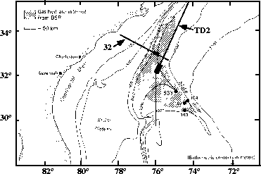
The data used in this study were recorded along two nearly perpendicular lines at the Blake Outer Ridge, offshore Florida and Georgia. A precise location of the lines can be seen in Figure map. The small rectangular boxes emphasize the parts of the lines used in this study. Both lines were acquired over deep water and in a region that is characterized by hydrate-bearing sediments.

 

map
Figure 1 Map of the Blake Outer Ridge area offshore Florida and Georgia, showing the location of the seismic lines 32 and TD2. The part of the lines used in this study are indicated by small rectangles. Map by Kvenvolden and Barnard (1983).

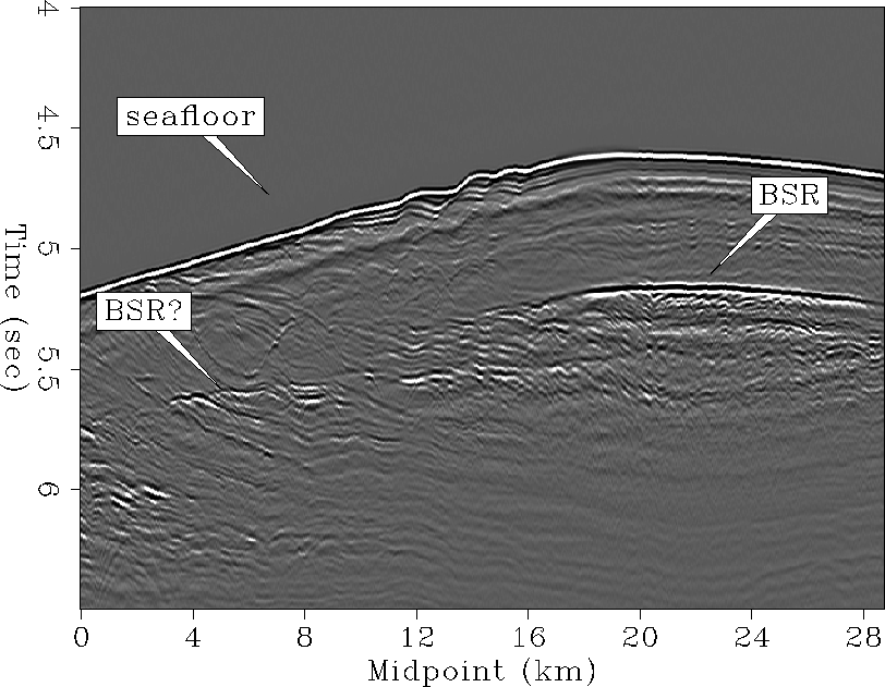
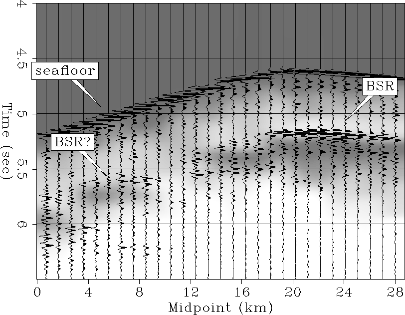
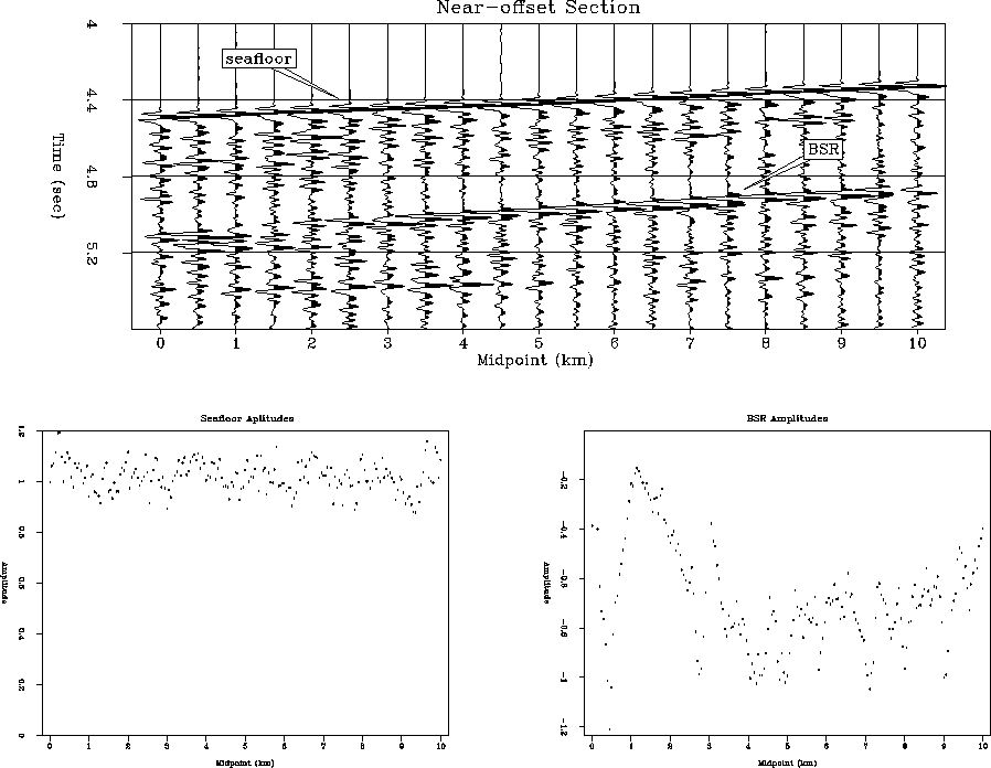
A stacked section of the data from line TD2 can be seen in Figure stack-td2-ann. The data contained approximately 600 shot points with a shot point interval of 50 meters. The northeast corner of the line is represented by midpoint 28, while the southwest corner is represented by midpoint 0. The stacked section displays a seafloor reflection at more than 4.5 seconds two-way traveltime, indicating a water depth of more than 3 kilometers. Between midpoint 17 and 28, a strong bottom simulating reflector parallels the seafloor at approximately 5.3 seconds two-way traveltime. In a small section above this strong BSR there is a ``quiet'' zone where no diffractions or reflections are visible. This might be caused by the presence of disseminated methane hydrate in this region. The strong BSR continuity is abruptly terminated at midpoint 17, coinciding with an increase in the seafloor dip. Immediately above the endpoint of the BSR, the seafloor topography appears to roughen, manifesting a ``bump-like'' structure. A possible explanation might be a variation in the pressure-temperature regime of the hydrate stability zone, thus causing the gas trapped inside to be released at this seafloor location. For midpoints less than 16, the BSR is considerably discontinuous and weak. It might possibly be identified between midpoints 12 to 16, and midpoints 4 to 8 because of some transversing, sedimentary structure. Since the BSR is not a structural boundary but parallels the seafloor by following a pressure-temperature relation, sediments with a dip different than the seafloor's may cut across the bottom simulating reflectors.

 

stack-td2-ann
Figure 2 Stacked section of line TD2.

 

stack-ann
Figure 3 Stacked section of line 32.

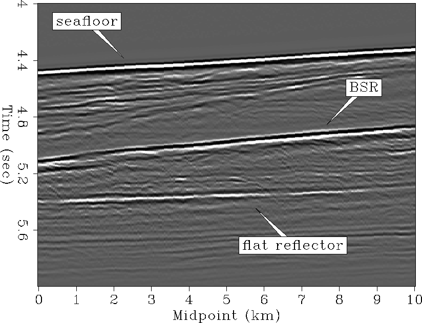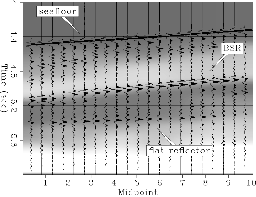
A stacked section of the part of line 32 used in this study can be seen in Figure stack-ann. A more precise description of the data can be found in Ecker and Lumley . The southeast corner of the line is represented by midpoint 0, while the northwest corner is represented by midpoint 10. As in line TD2, the seafloor reflection occurs at more than 4.4 seconds two-way traveltime, indicating a significant water depth. The section is characterized by a continuous, strong bottom simulating reflector at approximately 5.2 seconds two-way traveltime. Right above the BSR, there is a zone of amplitude blanking, possibly due to the presence of hydrate. A fairly bright reflection can be seen beneath the BSR, which is possibly indicative of the base of the gas-saturated sediments underlaying the hydrate (). Even though there are some reflection signals visible beneath the strong part of the BSR in the stacked section of line TD2 (Figure stack-td2-ann), there is no obvious evidence of a strong boundary between gas-saturated sediment and underlaying brine-saturated sediment along that line.

VELOCITY ANALYSIS ON LINE TD2

In order to determine the lateral and vertical variations of the hydrate and the possible underlying gas-saturated sediments, I performed a 2-D velocity analysis along line TD2.

Velocity analysis and preprocessing

Prior to the velocity analysis, the data were preprocessed. I first applied a time-varying spherical divergence correction. Subsequently, I performed a single-trace predictive deconvolution to suppress a ringing in the data induced by airgun bubbles. The deconvolved data were then bandpass-filtered to their original bandwidth to remove spurious deconvolutional high-frequency noise. Afterwards, I performed NMO stacking analysis along the entire line. Since the structure in the area is rather simple and the water depth is more than 3 kilometers, conventional NMO stacking velocity analysis was sufficient to obtain good RMS velocities. After the velocity analysis, normal moveout calibration was applied to the data. An additional static shift was used to account for a small non-hyperbolic, offset-dependent residual moveout. Subsequently, I obtained the final stacked section which was shown in the previous section (Figure stack-td2-ann).

Velocity analysis results

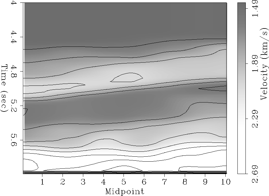
Using Dix's equation, I converted the obtained RMS stacking velocities into a physical interval velocity model. The estimated model for the entire line can be seen in Figure vint-td2. From midpoints 17 to 28, the model displays a significant increase in velocity up to approximately 1.95 km/s at 5.3 seconds two-way traveltime. Below 5.3 seconds traveltime, there seems to be a considerable velocity decrease to about 1.5 km/s. A slightly smaller velocity contrast is visible between midpoint 13 and 17. The velocity increases relatively quickly between midpoints 13 and 8, but there is no sharp velocity contrast visible from high to low velocity. For midpoints smaller than 8, the data are again characterized by a small low-velocity zone. However, it appears that the velocity does not decrease as much as previously, going down to only about 1.6 km/s. Simultaneously, the velocity increase above is not as pronounced, going up to about 1.85 km/s.

 

vint-td2
Figure 4 Interval velocity model for line TD2.

 

stack-td2-over-ann
Figure 5 Stacked section of line TD2 overlaying the interval velocity model.

The comparison between the stacked section and the interval velocity model is shown in Figure stack-td2-over-ann. It is obvious that the strong BSR between midpoints 17 and 20 coincides with the transition from significantly high P-wave velocity to considerably low velocity. This velocity behavior at the BSR supports the assumption of gas sediments underlying hydrate-bearing sediments in this region. The zone of a less pronounced velocity contrast between midpoints 13 and 17, and 4 and 8, seems to be associated with a possibly weak, discontinuous part of the BSR. The weak reflectivity of the BSR and the relatively smaller velocity contrast might suggest the presence of less hydrate and less free gas in this region or, possibly, a transition of a completely frozen hydrate state into a slightly more ``slushy'' state. Such behavior might be expected in the proximity of destabilization of the hydrate pressure-temperature regime. Between midpoints 8 and 13, the stacked section does not show any obvious reflection signals and there is no low-velocity zone visible in the data.

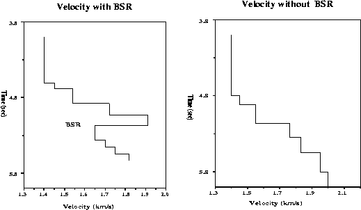
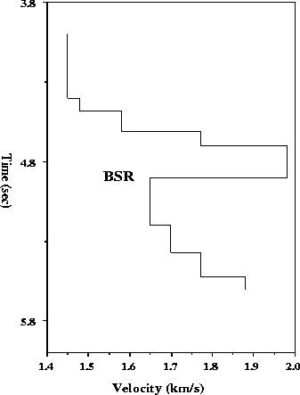
An average interval velocity model of the region characterized by a BSR and the region showing no BSR at all can be seen in Figure veltd2. The strong BSR is clearly associated with a high P-wave velocity of approximately 1.95 km/s in the hydrate section and an average low P-wave velocity of about 1.65 km/s in the underlaying sediments. On the other hand, the region showing no BSR reflection is characterized by a gradual velocity increase. The velocity increase does not seem high enough to justify the presence of hydrate in this zone. Consequently, the pressure-temperature regime associated with the hydrate stability field might be destabilized in this region, causing the possible transformation of frozen methane hydrate into free gas that could be released through the sediments. Reestablishement of sufficient pressure-temperature conditions close to midpoint 8 might lead to the renewed stabilization of the hydrate. An other possibility might be the change of methane source conditions. In case of local methane generation from organic material, this would imply the absence of a methane source between midpoints 8 and 13.

 

veltd2
Figure 6 Averaged interval velocity model for the region without BSR and the region with BSR.

VELOCITY ANALYSIS ON LINE 32

Following the 2-D velocity analysis on line TD2, I performed a similar analysis along line 32 to evaluate possible similarities in the behavior of the hydrate structure. Since line 32 is characterized by a continuous, strong BSR, I expect the velocity to show a velocity contrast comparable to the one observed along the BSR in line TD2.

Velocity analysis and preprocessing

Prior to the velocity analysis, I preprocessed the data similarly to those in line TD2. First, a time-varying spherical divergence correction was applied, which was followed by single-trace source wavelet deconvolution to regularize the source wavelet with offset. The deconvolved data were again bandpass filtered and subsequently used in a NMO stacking velocity analysis. Afterwards, a normal moveout correction was applied, as well as a careful amplitude calibration to reserve the true amplitude behavior. A more thorough description of the preprocessing steps can be found in Ecker and Lumley . The stacked section of the data so processed can be seen in Figure stack-ann.

Velocity analysis results

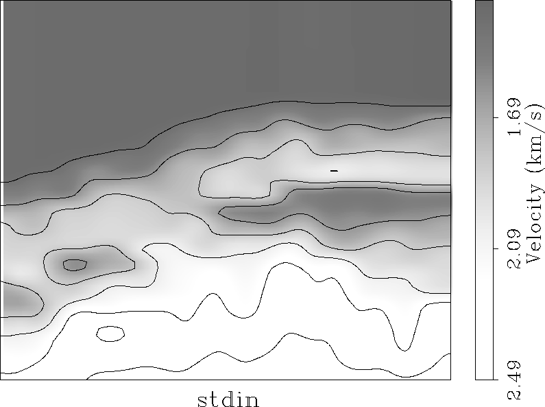
Using Dix's equations, I converted the RMS stacking velocities into a physical interval velocity model (Figure vint). The model shows a considerable velocity increase of approximately 1.95 to 2.0 km/s at around 5.2 seconds two-way traveltime along the entire line. The high velocity zone is underlain by a large zone of low P-wave velocity of approximately 1.6 km/s.

Comparison of the velocity model with the stacked section (Figure stack-over-ann) shows that the BSR is associated with the transition from high to low P-wave velocity. The strong increase in velocity above the BSR seems to parallel the upper boundary of the zone of amplitude blanking. This might be indicative of the presence of hydrate throughout a relatively large zone. It is also obvious that the flat reflector below the BSR seems to represent the bottom of the low-velocity zone underlaying the hydrate-bearing sediments. The considerable decrease in velocity suggests the presence of free gas in the layer, which agrees well with previous local results from this line ().

The velocity model appears to suggest the presence of free gas in the entire layer, in which case the flat reflector would be caused by the transition from gas-saturated sediment to brine-saturated sediment ().

 

vint
Figure 7 Interval velocity model for line 32.

 

stack-over-ann
Figure 8 Stacked section of line 32 overlaying the interval velocity model.

The average velocity model along the line is shown in Figure vel32. It is characterized by a significant increase in velocity above the BSR ( 1.95 km/s), and by a low-velocity zone of approximately 1.65 km/s below the BSR. A similar behavior could be observed in line TD2. However, contrary to line 32, line TD2 did not display such a strong reflection at the bottom of the low-velocity zone, possibly suggesting a more gradual velocity behavior there.

 

vel32
Figure 9 Averaged interval velocity model for line 32.

Reflection coefficient

In order to obtain additional information about the hydrate structure, I estimated the zero-offset seafloor and BSR reflection coefficient. These reflection coefficients will result in further constraints of the P-wave velocities and densities at the seafloor and the BSR. I estimated the reflection coefficients using the following relation by Warner :

$$R_{sf} \: = \:{ A_m \over A_p}$$ (1)

$$R_{BSR} \: = \: {A_{BSR} \over A_p} R_{sf}$$ (2)

where A_P is the maximum near-offset seafloor amplitude, A_m is the amplitude of the near-offset seafloor multiple and A_BSR is the maximum amplitude of the near-offset BSR. The seafloor reflection coefficient is represented by R_sf, and the BSR reflection coefficient is represented by R_BSR.

 

coef
Figure 10 The upper panel shows a near-offset seismic section of line 32. The lower panel shows the amplitude picks from the seafloor reflection(left) and the BSR reflection(right).

The upper panel of Figure coef shows a section of the near-offset seafloor and BSR amplitudes. The seafloor amplitude seems to stay approximately constant along the entire line, while the BSR amplitude appears to be characterized by some lateral variations. Between midpoints 1 and 3, the BSR reflection displays a significant decrease in amplitude compared to the remainder of the section. Picking the peak amplitudes along the seafloor and the BSR yields the amplitude trends shown in the lower panel of Figure coef. The average seafloor amplitude can be determined to approximately 1.05 $\pm$ 0.1. The BSR picks between midpoints 3 and 10 can be averaged to an amplitude of approximately -0.8 $\pm$ 0.2. Prior to midpoint 3, the BSR amplitude is subject to large variations. Using the averaged seafloor and BSR amplitudes, I estimated a seafloor reflection coefficient of approximately 0.17 $\pm$ 0.01 and a BSR reflection coefficient of -0.12 $\pm$ 0.02. This BSR reflection coefficient is only representative of the part of the line characterized by the large BSR reflectivity.

Modeling

In order to determine a preliminary P-wave and density model that can recreate the near-offset amplitudes of the structure, I combined the information given by the reflection coefficients and the average interval velocity model. After generating velocity and density models that are constrained by both pieces of information, I performed a 1-D elastic amplitude modeling of the near-offset traces using a Thompson-Haskell method. The resulting near-offset response was then compared with the amplitude response representative for the line.

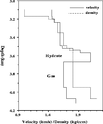
The BSR and seafloor reflection coefficients, estimated in the previous section, provided additional constraints to the average velocity model determined in the velocity analysis. Furthermore, they gave some insight into the possible density behavior at the transition from hydrate-bearing sediments to gas-saturated sediments. A velocity and density model that might explain the amplitudes in the original data is shown in Figure endvel. In order to fulfill all constraints given, the P-wave velocity in the hydrate is required to increase to approximately 2.1 km/s. The thickness of the hydrate section seems to be about 80 meters. The hydrate is underlain by slow-velocity zone of 1.65 km/s and a thickness of approximately 300 meters. The density is required to stay approximately constant across the transition from hydrate to gas. This velocity behavior is strongly supported by results obtained through ray modeling and P- and S-impedance migration/inversion presented in SEP80 ().

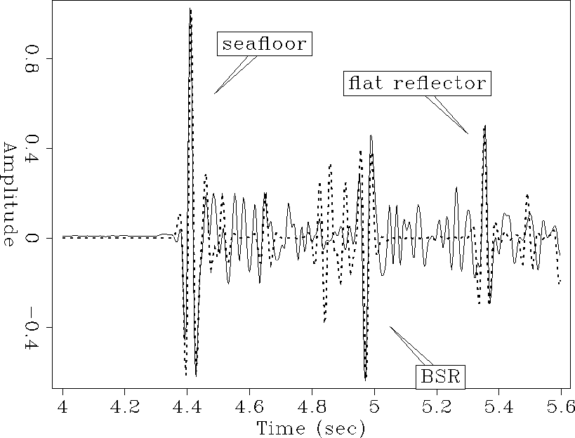
The near-offset trace resulting from this model is compared with the near-offset amplitude behavior of the original data in Figure model. The original data trace is given as a solid line, while the modeled trace is displayed using a dashed line. It is obvious that the model could successfully recreate the seafloor amplitude, the BSR amplitude and the amplitude of the ``flat reflector''. However, the model created some significant reflection amplitudes preceding the BSR reflection that were not present in the original data. This probably suggests the presence of a gradient velocity model rather than a blocky model.

 

endvel
Figure 11 Final P-wave velocity and density model.

 

model-ann
Figure 12 Modeled near-offset trace compared with an original near-offset trace. The modeled trace is indicated by the dashed line.

CONCLUSIONS

A detailed 2-D velocity analysis was performed on two approximately perpendicular seismic lines from the Blake Outer Ridge, offshore Florida and Georgia. The inferred interval velocities clearly showed that regions of strong BSRs are characterized by a considerable increase in P-wave velocity in the hydrate-bearing sediments overlaying a low-velocity gas zone. Weaker BSR reflections seem to be associated with a similar, but slightly smaller velocity contrast. Loss in the BSR reflectivity and simultaneous decrease in the observed velocity contrast appeared to be related to changes in the temperature-pressure regime of the hydrate stability zone or to the absence of a local methane source.

Subsequent estimations of the BSR and seafloor reflection coefficients along line 32 resulted in additional constraints for the P-wave interval velocity and density in the vicinity of the BSR. Combination of both the reflection coefficient and average velocity information in a 1-D modeling approach showed that the hydrate zone of line 32 is characterized by a velocity of approximately 2.1 km/s and a thickness of 70 meters. It seems to overlay a 300 meter thick gas-saturated sediment zone with a velocity of 1.65 km/s. The density is required to stay approximately constant across the transition zone. This result agrees well with previous results obtained by Ecker and Lumley .

ACKNOWLEDGMENTS

I would like to thank Myung Lee, Bill Dillon and Keith Kvenvolden from the USGS for providing me with the seismic section from the Blake Outer Ridge. I would also like to thank David Lumley for many helpful discussions and suggestions. Furthermore, I am grateful to Mark Van Schaack and Yizhaq Makovsky for their assistance in installing the PROMAX geometry.

[MISC,SEP]