Flying over the Ocean Southeast of Madagascar

Christine Ecker and Arnaud Berlioux

christin@sep.stanford.edu, arnaud@sep.stanford.edu

ABSTRACT

Satellite measurements from the Southwest Indian Ridge provide information about the local ocean topography along both ascending and descending tracks. We present a weighted least-squares approach to combine the information given along these two measurement directions, thus obtaining a dense altitude coverage. High-frequency, spiky noise along the tracks is eliminated by additional weighting of the derivatives of the initial residuals. After having obtained the optimal altitude fit to the crossing data, we illuminate the local seafloor features using a set of first-order derivative filters. The results show high image resolution, indicating effective noise removal.

INTRODUCTION

Information about global ocean topography can be inferred from advanced radar altimetry measurements of earth satellites. These satellites orbit around the earth in north-flying and south-flying tracks which appear to drift westward due to the earth's rotation. They measure both the rather high-frequency seafloor topography and the low-frequency sea surface altitude which is influenced by weather changes, tides and ocean currents at the time of the recording. The high-frequency seafloor component can be separated from the masking low-frequency trend by taking the time derivative along the tracks. In order to obtain an optimal altitude coverage of a specific area, the measurements along those two non-orthogonal satellite track directions must be combined. This approach might be directly applicable to the frequently occurring problem of tying inconsistent seismic lines to obtain higher information density for 3-D surveys.

In this paper, we present a weighted least-squares approach to combine track measurements from the Southwest Indian Ridge in the Indian Ocean. The method is based on an approach proposed by Claerbout . The weighting function which is applied to each track is represented by a derivative operator along the tracks to eliminate the low-frequency data trend. Failure to remove this component would cause large residuals for the least-squares fitting of crossing tracks that are inconsistent at the crossing point. Since the data appear to be contaminated by high-frequency, spiky noise, we additionally weight the derivative of the starting residuals. Subsequently, we convolve the resulting altitude data with a set of first order derivative filters in different directions to illuminate the local features.

SATELLITE DATA

The data consist of two sets of altimetry measurements recorded by the satellite GEOSAT above parts of the Southwest Indian Ridge in the Indian Ocean. The two data sets correspond to the ascending and descending paths of the satellite, thus representing two crossing track data sets. Both ascending and descending tracks have a spatial interval of approximately 2.8 km and cover an area between latitude $30^{\circ} S$and $40^{\circ} S$ and longitude $40^{\circ} E$ and $70^{\circ} E$.A gravity anomaly map of the Indian Ocean, which was given to us by Professor David Sandwell, University of California in San Diego, (Figure map) displays the interesting seafloor topography in this region. The part of the Southwest Indian Ridge structure covered by the satellite measurements is indicated by the small rectangular area. Both the ascending and the descending data files consist of seven columns of 32 bit integers each of which include more than 220,000 measurements. The columns correspond to the following parameters:

 

map
Figure 1 Gravity anomaly map showing the seafloor topography of part of the Indian Ocean. The small rectangular area indicates our area of interest.

1.

time in seconds since the first day of the year the satellite was launched,

2.

the continuation of time in microseconds,

3.

the geodetic latitude in microdegrees,

4.

the longitude in microdegrees,

5.

the sea surface height above the reference ellipsoid with corrections applied, in millimeters,

6.

the sea surface slope in micrometers per seconds (time derivative between two measurements of the height.)
N.B.: the first element is the number of points in a pass,

7.

sum of all the corrections.

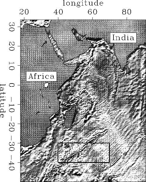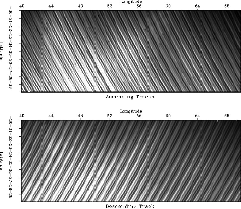
Figure tracks shows the altitude data for both the ascending and descending satellite tracks which were interpolated to a regular grid of 100 points along the vertical axis and 240 points along the horizontal axis. Although the single tracks can be clearly discriminated, the coverage of the ridge region is relatively dense in both directions. The recorded data corresponds to the height difference between the sea surface and the reference ellipsoid at the respective locations. Regions of high relief are plotted as white, while regions of low relief appear dark. The gravitational attraction of sea mountains, trenches and ridges beneath the sea causes the sea surface altitude to vary globally, thus mirroring the seafloor topography. However, in Figure tracks the seafloor features are not visible. They are masked by a low-frequency trend of the sea surface altitude induced by changes in weather, tides and ocean currents.

 

tracks
Figure 2 Original altitude data.

COMBINATION OF THE TRACKS

In order to obtain higher information density/data coverage in the region covered by the satellite measurements, we attempt to combine the data information given along the ascending and descending tracks. This is accomplished using a weighted least-squares approach as described by Claerbout . In this approach, we use conjugate gradients to find the best-fitting altitude h mapped on a regular grid by combining the two irregularly-sampled data vectors d_a (ascending tracks) and d_d (descending tracks). The following equations describe the problem formulation:

$$0 \: \approx \: r_a\: =\: \frac{\partial }{\partial t_a}\: ( L_a \: h - d_a)$$ (1)

$$0 \: \approx \: r_d\: =\: \frac{\partial }{\partial t_d}\: ( L_d \: h - d_d)$$ (2)

where $\frac{\partial } {\partial t_a}$ is the derivative along the ascending tracks and $\frac{\partial }{\partial t_d}$ is the derivative along the descending tracks; r_a is the ascending residual, while r_d is the descending residual. The linear interpolation operators L_a and L_d put the data on a regular grid.

The derivative operators correspond to weighting operators along the data recording trajectories. They remove the low-frequency data trend caused by tides or ocean currents. Failure to account for this trend would result in significantly large residuals for the fitting of crossing tracks that are inconsistent at the point of crossing.

In order to obtain an optimal altitude h, we must eliminate the high-frequency, spiky noise that appears to contaminate the data. Since the noise is more prominent after the derivative is applied along each track, we attempt to remove it by weighting the initial ascending and descending residuals r_a0 and r_d0. Since the noise spikes are easy to identify in these data, we apply a weighting function which cuts off all energy bursts above a mean value $\overline{r}$.

$${r_a}_0 \: =\: W \: \frac{\partial }{\partial t_a} \:( \:- d_a )$$ (3)

$${r_d}_0 \: = \: W \: \frac{\partial }{\partial t_d} \:( \: - d_d )$$ (4)

with

$$W = \left\{\begin{array} {ll} 0 & \mbox{if $ \vert\frac{\pa... ...\overline{r}$} \\ 1 & \mbox{ otherwise.} \end{array} \right.$$ (5)

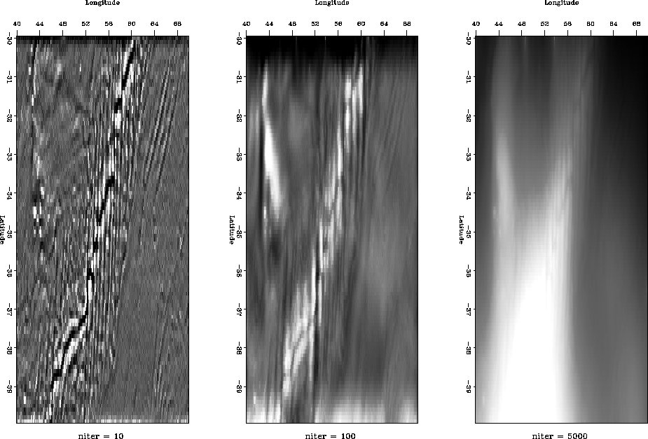
Figure iter shows the optimal altitude h after 10, 100 and 5000 iterations. After only 10 iterations, the altitude displays none of the low-frequency behavior of the original data. It is rather characterized by high-frequency features resembling a ridge structure as shown in the gravity anomaly map (Figure map). This is due to the fact that we use the derivatives along the tracks as weighting operators. They eliminate the low-frequencies in the data, thus minimizing the possible inconsistencies between crossing data points. Therefore, if too few iterations are applied, the low-frequency trend of the original data will not be recreated. The more iterations are incorporated into the least-squares fitting, the more low-frequencies are included into the solution altitude. After 100 iterations, the ridge structure has considerably faded, and after 5000 iterations the altitude represents a good fit to the original ascending and descending data shown in Figure tracks.

 

iter
Figure 3 Least-squares fit of the altitude h after 10, 100 and 5000 iterations.

ILLUMINATION OF THE ALTITUDE DATA

After having combined the altitude information given by both the ascending and descending satellite measurements, we attempt to derive an image of the local seafloor topography from the new altitude data. Since the topography information is masked by a low-frequency trend, we convolve the data with a set of first-order derivatives to illuminate the seafloor features. These four filters consist of a vertical filter, a horizontal filter and two diagonal filters. One is taken at $45^{\circ}$ which is approximate in direction of the ascending tracks, while the other one runs at $45^{\circ}$ in approximately the direction of the descending tracks. The filters are represented by:

$\left(\begin{array} {cc} 1 & . \\ -1 & . \end{array}\right)$,$\left(\begin{array} {cc} 1 &-1 \\ . & . \end{array}\right)$,$\left(\begin{array} {cc} 1 & . \\ . &-1 \end{array}\right)$,$\left(\begin{array} {cc} . &1 \\ -1 &. \end{array}\right)$

Figure asc-deriv shows the illumination of the seafloor in the direction of the ascending tracks. The upper frame is the result of taking the derivative along the original ascending data tracks. The single tracks are clearly visible, as well as some scattered noise bursts. A ridge structure strikes diagonal from SW to NE and seems to be translated by several N-S striking transform faults. To the west of the ridge, a small topographic feature is noticeable, but quite difficult to recognize. The lower frame of Figure asc-deriv represents the result of the convolution of the solution altitude h with a diagonal filter in the direction of the ascending tracks. Although the original track direction is not exactly $45^{\circ}$, it can be considered a good approximation. It is obvious that the use of the solution altitude results in a significantly increase of the image resolution. The combination of the ascending and descending data has improved the data quality, as well as effectively removed the noise spikes. It is easy to identify both the transform faults translating the ridge structure and the sea mountain west of the ridge.

 

asc-deriv
Figure 4 Illumination of the seafloor features in the ascending direction. The upper frame respresent the derivative along the tracks in the original ascending data set. The lower frame illuminates the topography of the solution altitude using a $45^{\circ}$ filter in approximately the ascending direction.

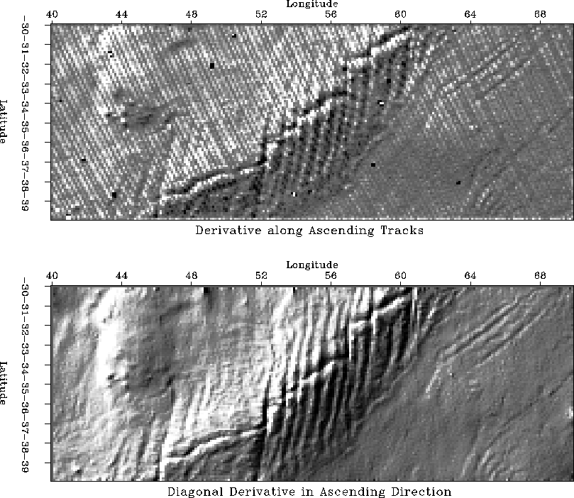Figure desc-deriv displays the illumination of the seafloor in the direction of the descending tracks. As before, the upper frame represents the derivative taken along the tracks of the original descending data set. The lower frame illuminates the seafloor of the altitude data after combining ascending and descending data. Like the illumination in the ascending direction, this Figure shows the improvement in image quality and resolution of the data combination over the original data set. It also indicates the successful elimination of noise bursts in the data. As a result of the use of a filter in the descending direction, the actual ridge structure appears much dimmer than in Figure asc-deriv and is characterized by less relief. The most prominent features are the N-S striking transform faults. The westward sea mountain, illuminated from the opposite side than before, is also obvious.

 

desc-deriv
Figure 5 Seafloor topography for illumination along the descending direction. The upper frame is the result of the derivative taken along the descending tracks of the original data. The lower frame shows the seafloor features after illumination with a diagonal filter in approximately the descending direction.

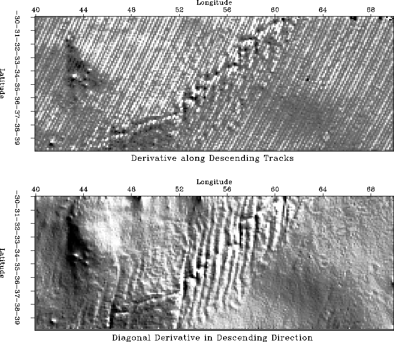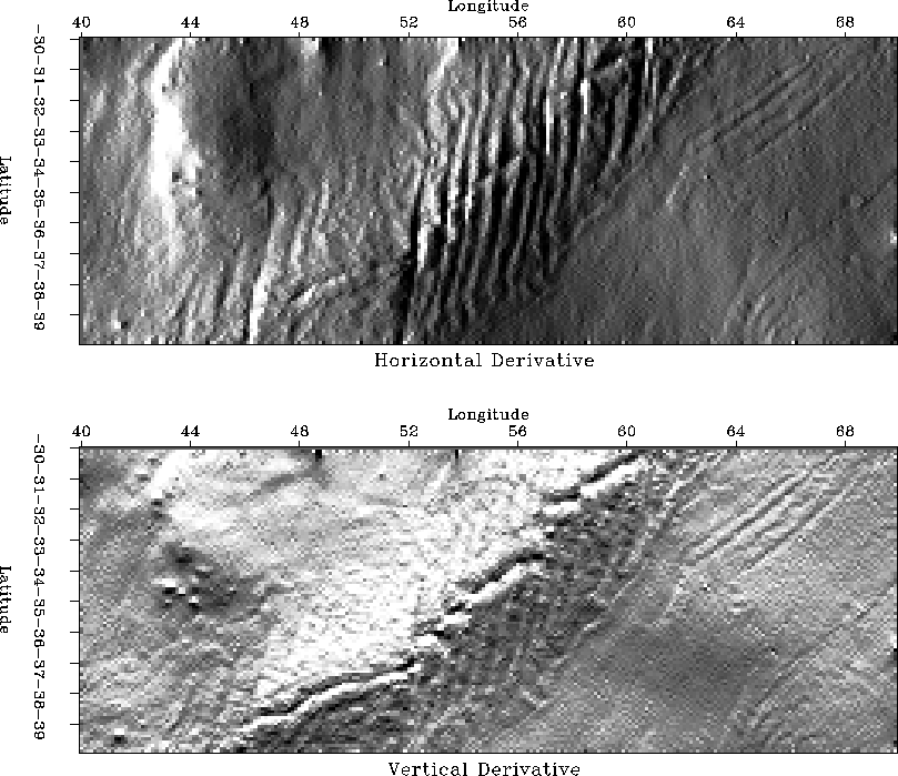
Figure deriv shows the result of the illumination of the seafloor features using a horizontal and a vertical filter. Both filters were convolved with the solution altitude h after combining the ascending and descending data set. As in the illumination with a diagonal filter in the descending direction, convolution with a horizontal filter does not show much of the ridge structure itself, but results in proment N-S striking transform faults. The illumination using a vertical filter, on the other hand, clearly accentuates the ridge structure and suppresses the transform faults entirely. Contrary to the horizontal filter, the vertical filter displays less ``shadow zones''.

 

deriv
Figure 6 Illumination of the seafloor features using a horizontal filter (upper frame) and a vertical filter (lower frame).

FUTURE RESEARCH

Besides the two data sets presented in this paper, we are in the possession of two more data sets which cover the area between latitude $20^{\circ} S$and $30^{\circ} S$ and longitude $40^{\circ} E$ and $70^{\circ} E$. These two data sets are directly adjacent to those shown her and also consist of ascending and descending satellite track measurements. However, their spatial sampling interval between tracks is considerably larger, thus resulting in a relatively sparse coverage of the region.

As a future research opportunity, it might be interesting to try to determine the missing information in these data sets. One possibility might be the determination of a 2-D prediction error filter in the already known region defined by the data sets that were combined in this study. This PEF might then be applied to the combined, sparse data tracks. In this case, a region of dense coverage would be used to obtain information about a region of sparse data coverage. Another possibility might be to recreate the data by using two 1-D prediction error filters determined directly along each track, as proposed by Jon Claerbout in his book Three-Dimensional Filtering. In this case, a dense coverage of a region would not be necessary.

CONCLUSIONS

Ascending and descending satellite measurements above part of the Southwest Indian Ridge were used to demonstrate a weighted least-squares technique to combine the given data information. This was done to obtain a higher information density and thus an optimal data coverage. The problem of high-frequency, spiky noise contamination in both data sets was solved by applying an initial weighting function to the starting residuals. Our results show that the combination of the two data sets resulted in an considerable increase of image resolution. The dat quality improved significantly and the noise burst could be effectively removed.

ACKNOWLEDGEMENTS

We would like to thank Professor Jon Claerbout for his valuable ideas and advise. We also thank Professor David Sandwell, the University of California in San Diego, for providing Professor Claerbout with the Seasat dataset.

[MISC,SEP]