

![[*]](http://sepwww.stanford.edu/latex2html/prev_gr.gif)


ABSTRACTIt is well known that the inverse problem of estimating interval velocities from reflection data is poorly constrained in 2-D. We show that the interval velocity estimation problem in 3-D is much better constrained when the velocity function is estimated by jointly inverting the data collected along multiple offset-azimuth, even when the azimuth range is fairly limited. We extend to 3-D the linear operator presented by () for relating stacking velocities with interval velocities. We then apply a Singular Value Decomposition (SVD) analysis to the derived operator. This analysis suggests that methods that take advantage of the azimuth range in the data should yield better velocity functions than currently used velocity estimation methods that neglect the additional information provided by multi-azimuth coverage. |
In the last 10 years numerous methods have been proposed for estimating interval velocity from reflection data in two-dimensions. Toldi presented a method for inverting stacking velocities. Etgen used residual migration and Biondi used beam stacking in conjunction with prestack migration in iterative inversion schemes to estimate the velocity model. All these methods suffer from the common reflection tomography problem that the inverse operator has a large null space (, ) due to some components of the velocity model having no, or very small, effect on the travel-times of the data.
In the case of 3-D data there is a potential to improve the inversion process by exploiting the fact that data is collected along several offset-azimuths. Common practice is to ignore the azimuth at which the data was collected or try to account for differences in recorded stacking velocities by introducing an anisotropic component to the velocity field. Seldom is the azimuth at which data is collected considered in inverting for interval velocity. If we take the approach that the varying azimuths at which data is collected is another source of information for estimating interval velocity, rather than a hindrance, there is a potential to improve the inversion process. We show that in 3-D the interval velocity estimation problem is much better constrained when the data recorded along multiple azimuths is inverted for simultaneously.
We extend Toldi's 2-D interval velocity estimation from stacking velocities to 3-D, taking into account the azimuth in which the data was collected. By analyzing the singular values of the SVD, we show that the problem becomes fairly well defined when the data is recorded along at least two azimuths; the wider the azimuth range the better. However, we show by applying the method on a series of synthetics, that the multi-azimuth approach is of great help in improving the resolution and reliability of the velocity estimation even when the range of azimuths is limited, as is in modern multi-streamer marine acquisition.
THEORY
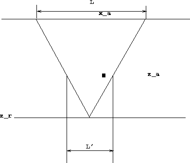
3-D data is routinely collected along several azimuths. For land surveys, CMP's contain information from a wide range of azimuths. In the case of marine surveys, state of the art a few years ago in marine acquisition () resulted in CMP's whose azimuth information that varied greatly from CMP to CMP, and was extremely limited in range. As time progresses there is a growing desire to increase fold, CMP coverage, and azimuth coverage. As a result we are seeing more cables, wider cable offset, and more overlap in boat paths producing wider and more uniform azimuth coverage. When velocity varies laterally, the azimuth at which data is collected has a significant effect on measured stacking velocities. Figure azimuth shows the stacking velocities that would be measured from a planar reflector below a Gaussian anomaly as function of the azimuth at which the data was collected.
 |
In the case of a flat layered earth and assuming no ray bending, perturbations in stacking velocities can be approximated as the linear operation:
| (1) |
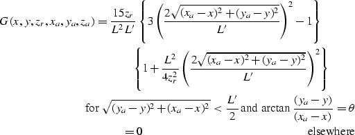 |
||
| (2) | ||
| (3) |
| (4) |
 |

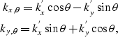
sheadFourier Analysis Considering the problem in the wavenumber domain provides two significant advantages over a strict spatial domain analysis. First, if we bring the problem into the wavenumber domain each wavenumber can be considered independently (making computationally possible the SVD inversion of G). In addition a Fourier domain analysis better illustrates why considering multiple azimuths is advantageous. The wavenumbers who have a low/zero amplitude response will not invert properly, especially when we consider noise. With multiple azimuths, the number of wavenumbers who have low amplitudes (determined by summing of the amplitude response at each azimuth) is greatly reduced. To account for multiple azimuths we need to perform an azimuth rotation. This is accomplished in the wavenumber domain by:
 |
(5) | |
| (6) |
![\begin{eqnarray}
G(\vec k_{\theta},z_r,\theta,z_a) =
{15z_r \over L^2 k_{x,\the...
...left[(6+10c)k_{x,\theta}^2-72ck_{x,\theta}\right]\cos k_{x,\theta}\end{eqnarray}](img9.gif) |
||
| (7) |
Where c is equal to:
| (8) |
| |
(9) |
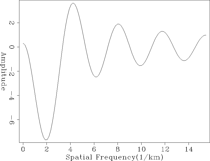
Figure transfer shows ![]() at a fixed
at a fixed ![]() , ky,
zr and za.
The zeros, and all the wavenumbers close to them represent spatial wavelengths
that can not be retrieved in the inversion process for a single azimuth
(the
inverse of
, ky,
zr and za.
The zeros, and all the wavenumbers close to them represent spatial wavelengths
that can not be retrieved in the inversion process for a single azimuth
(the
inverse of ![]() would go to infinity). The single azimuth
problem is helped somewhat with multiple
zr, because the zeros of
would go to infinity). The single azimuth
problem is helped somewhat with multiple
zr, because the zeros of ![]() are a function of the
effective cable length, but as Figure bad shows the inversion of
are a function of the
effective cable length, but as Figure bad shows the inversion of
![]() for a single azimuth still has
significant artifacts even when stacking velocity is measured at several
reflectors. Part of this can be attributed to the first zero
of
for a single azimuth still has
significant artifacts even when stacking velocity is measured at several
reflectors. Part of this can be attributed to the first zero
of ![]() , which is close to the origin (low spatial wavelengths),
and therefore is not greatly affected
by multiple reflectors and the resulting stretch.
, which is close to the origin (low spatial wavelengths),
and therefore is not greatly affected
by multiple reflectors and the resulting stretch.
 |


 |
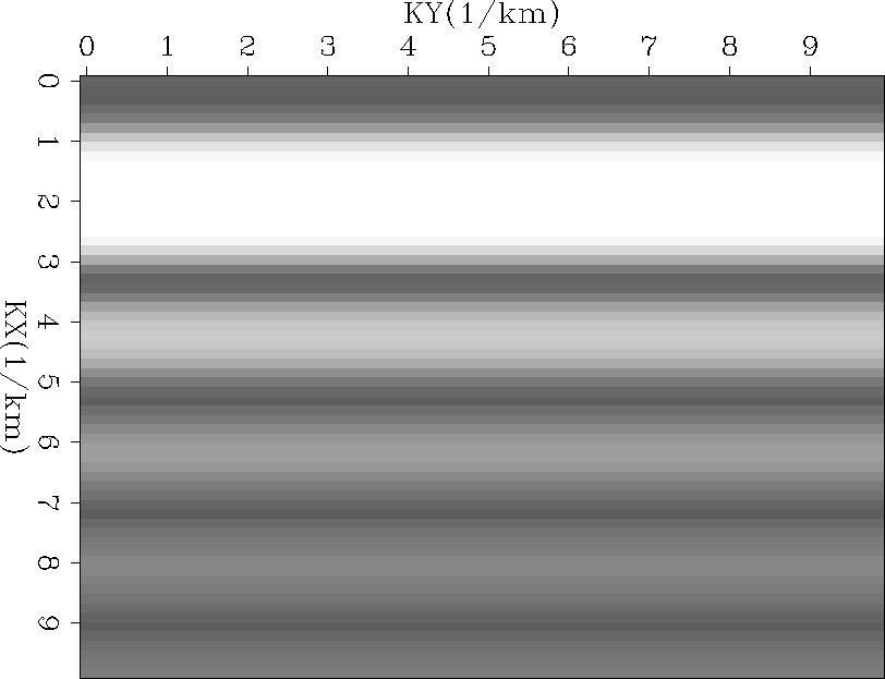
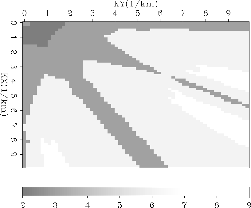
The low spatial wavenumber problem is
significantly reduced when multiple azimuths are considered.
To understand why, imagine stacking velocities measured on a planar 3-D surface
below a small velocity perturbation in an otherwise homogeneous earth.
In the first case the data is collected along a single azimuth and
the stacking velocity is then 2-D Fourier transformed.
In the second, the data is collected along three different azimuths and the
amplitude response of the Fourier transform of the corresponding stacking
velocity measurements are summed.
Figures Fourier and fouriercombo
show the resulting 2-D Fourier sections. In each plot the low values (dark)
represent spatial wavenumbers of the stacking velocity model
that are insensitive to the interval velocity model. As Figure
fouriercombo
shows, the number of spatial wavenumbers with low values is significantly
reduced.
This is a qualitative analysis of the the effect that multiple azimuths have on
the
characteristics of ![]() . In the next section we will show a more
rigorous one, using the SVD of
. In the next section we will show a more
rigorous one, using the SVD of ![]() .
.
 |
 |
Inversion
As stated earlier, we are not interested in the forward operation, instead we are
attempting to obtain interval velocities.
The interval velocity function can be estimated by
inverting equation (9).
In general, the rank of the matrix ![]() is lower than
the dimensionality of the unknown vector (
is lower than
the dimensionality of the unknown vector (![]() ),
and thus
),
and thus ![]() is not exactly invertible, illustrated by the large side
lobes in Figure bad.
There are two main reasons for the rank deficiency of
is not exactly invertible, illustrated by the large side
lobes in Figure bad.
There are two main reasons for the rank deficiency of ![]() .First, the number of data points (rows)
is usually lower than the number of unknowns (columns).
Second, even if enough reflectors and/or
azimuths were present,
.First, the number of data points (rows)
is usually lower than the number of unknowns (columns).
Second, even if enough reflectors and/or
azimuths were present, ![]() would be still
rank deficient because of fundamental velocity ambiguities
along the vertical axis.
We are however interested in an approximate inverse
of
would be still
rank deficient because of fundamental velocity ambiguities
along the vertical axis.
We are however interested in an approximate inverse
of ![]() , not in its exact inverse.
For practical purposes,
the quality of the velocity estimation can be greatly improved
if the null-space of
, not in its exact inverse.
For practical purposes,
the quality of the velocity estimation can be greatly improved
if the null-space of ![]() is reduced; we will show
that this happens when data with multiple azimuths
are considered.
is reduced; we will show
that this happens when data with multiple azimuths
are considered.
To analyze the property of ![]() , and of its inverse
we will perform a Singular Value Decomposition (SVD)
of the matrices
, and of its inverse
we will perform a Singular Value Decomposition (SVD)
of the matrices ![]() at each
wavenumber
at each
wavenumber ![]() and study their singular values and
singular vectors.
We will also use the SVD of
and study their singular values and
singular vectors.
We will also use the SVD of ![]() to invert it in
some interesting cases.
SINGULAR VALUE DECOMPOSITION OF
to invert it in
some interesting cases.
SINGULAR VALUE DECOMPOSITION OF ![]() A rectangular matrix, such as
A rectangular matrix, such as ![]() , can be
decomposed by SVD into
, can be
decomposed by SVD into
| |
(10) |
Once the SVD of a matrix is computed, its least-square inverse, or pseudoinverse is simply computed by,
| |
(11) |
| |
(12) |
SVD Analysis of ![]()
To analyze the properties of ![]() and of its pseudoinverse
we introduce the concept of effective rank of
and of its pseudoinverse
we introduce the concept of effective rank of ![]() as a
function of the wavenumbers.
The concept of effective rank of a matrix is
linked to the concept of condition number ().
The condition number is defined
as the ratio between the largest and the smallest singular values.
When inverting real data, matrices with too large of a
condition number are effectively rank deficient;
an upper limit must be set on the condition number.
The effective rank of a matrix is equal to the
order for which the ratio between
the largest singular value and the singular value of that order,
is less than the set upper limit on the condition number.
as a
function of the wavenumbers.
The concept of effective rank of a matrix is
linked to the concept of condition number ().
The condition number is defined
as the ratio between the largest and the smallest singular values.
When inverting real data, matrices with too large of a
condition number are effectively rank deficient;
an upper limit must be set on the condition number.
The effective rank of a matrix is equal to the
order for which the ratio between
the largest singular value and the singular value of that order,
is less than the set upper limit on the condition number.
Figure Rank-1 show the effective rank of the inverted matrix at each wavenumber when stacking velocity is measured along a single azimuth. At almost all wavenumbers the effective rank of the matrix is three, with small portions of the data going as low as two. When three azimuths at 60 degrees are considered in the inversion problem the effective rank, and therefore the inversion is significantly improved. Figure 3dview2 illustrates this point, few spatial wavenumbers have ranks of two or three, while many have effective ranks as high as nine. For computing the effective rank we have set the upper limit on the condition number to be equal to 10.
 |
SYNTHETIC MODEL TESTS
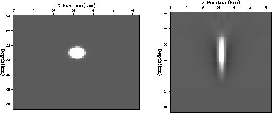
To test the effectiveness of the method we tested it on two models. We first apply the forward operator (equation 7) on the interval velocity model and then attempted to recover the interval velocity model by applying the damped inverse, equation (12). In each case we used an interval velocity model that was, 6.4 km in each direction (x, y, and z), sampled every 100 m, and cable length of 2 km.
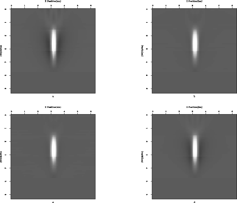
For our first test we placed a Gaussian velocity blob within a uniform half space. The blob had an approximate radius of 300 m and was centered at a depth of 2.5 km in the model of the survey. Stacking velocities were measured (by applying G to the interval velocity model) at three reflectors, two bounding the anomaly and one significantly below. Figure bad shows a 2-D slice through the Gaussian blob and the result of the inversion when stacking velocities are measured along one azimuth. We then attempted the inversion with multiple azimuths. Figure gauss.tot shows the inversion result when stacking velocities are measured along: one azimuth; two azimuths at 90 degree (common land survey design); three azimuths at 60 degrees; and three azimuths at 8 degrees (marine survey). As expected the result with three azimuths at 60 degrees is superior, but note the significant improvement over the one azimuth inversion for both the land and marine simulation. The blob is better constrained in the horizontal direction, and shows improvement in the vertical direction. In addition the artifacts evident in the one azimuth approach are reduced, and the recovered amplitudes better approximate the starting model.
 |
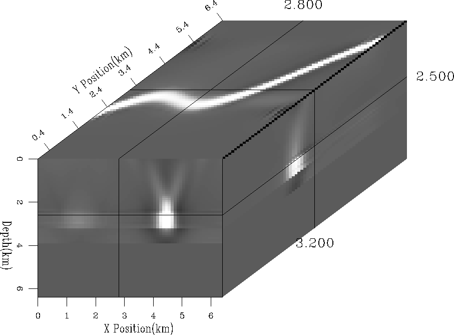
Buried River Channel Model
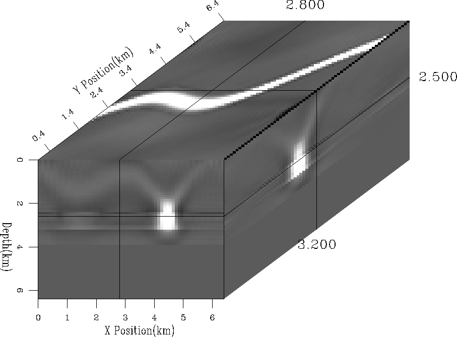
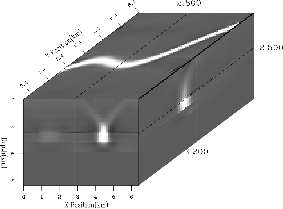
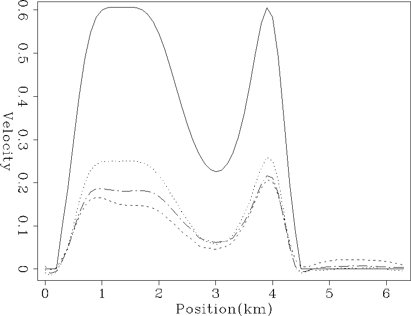
Our second test tried to invert for a buried river channel, Figure river. For the test, we added to a uniform half space, a velocity anomaly, with an approximate width of of 1 km and depth of 400 m. We simulated measured stacking velocities at 3 depths, one immediately above the river and two below (at intervals of 700 m). Figure chanel1 shows the result of the inversion along 1 azimuth, while Figure chanel3 shows the improvement when stacking velocities are measured along 3 azimuths at 60 degrees, and Figure chanel3b the result when the azimuth range is limited. All three methods successfully located the center of the river channel, but, again, when the multiple azimuths are considered the lateral extent of the anomaly are much better defined along with improved recovery of amplitudes, evident when amplitudes are compared along an arbitrary horizontal line (Figure amplitude).
 |
 |
 |
 |
 |
CONCLUSIONS
In this paper we present a 3-D extension of a common 2-D interval velocity estimation scheme from stacking velocities. The method uses the multi-azimuth component of 3-D surveys to reduce the null space inherent in the inversion process. We show that the inversion scheme is effective in reducing the null space by analyzing the effective rank of the forward operator. The method is then tested on a series of synthetic models. The test on the synthetic models show significantly improves the inversion result even when azimuth range is limited. The resulting interval velocity model is both improved in horizontal and vertical resolution. FUTURE WORK
In the future we plan to further test our current scheme and to apply what we have learned in this problem to further enhance our ability to estimate interval velocity in 3-D. As a first step we plan to test the current method using 3-D ray tracing to calculate travel times (and from that stacking velocities), instead of applying the forward operator to calculate stacking velocities. We also plan to test the current method on real data which has a gentle dip. And eventually to generalize the method to account for 3-D dips. Finally, the success of the method, indicates that other 2-D interval velocity estimation methods, might be extended into 3-D in a similar fashion, further improving velocity estimation. [bob,SEP,MISC,EAEG,GEOTLE,geophysics]