Stacking and migration of Oseberg data

Li Teng

Author has no known email address

ABSTRACT

This paper describes methods of stacking and post-stack migration that I used with a data set from Oseberg field. CMP(common midpoint) bins are used for brute stack to simplify the stacking procedure. Both two-pass 3-D post stack migration and Ristow's four-way splitting method are applied to migrate the stacked data. The result of four-pass migration doesn't show significant improvement over the two-pass result because brute stack, linear interpolation and other approximation.

Depth extrapolation of the one-way wave equation in three dimensions can be carried out using the splitting technique. Splitting in three dimensions is based on an approximation that enables the full 3-D operator to be realized by applying the 2-D operator along x for all y and then along y for all x. This technique yields an operator that is anisotropic, with the greatest error at the 45 degree azimuth from the x and y axes. Ristow suggested a four-pass method to compensate for the anisotropic errors by applying a finite-difference operator along the two conventional axes and the axes rotated to the 45 degree azimuth from the original axes.

To test the applicability of four-pass post-stack depth migration to real data, I processed the 3-D marine seismic data acquired over the Oseberg field in the North Sea. The original data I have are deconvolved shot gathers along eighteen parallel seismic lines. There are three primary stages in seismic data processing (): deconvolution, stacking, and migration. To get a rough image of the subsurface geological structures, I first applied CMP(common midpoint) bin stacking. I then applied two-pass and four-pass post-stack migration to the stacked section on the CM-5 machine to compare the results.

PRESTACK DATA AND STACKING

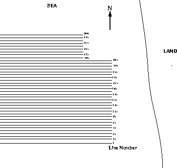
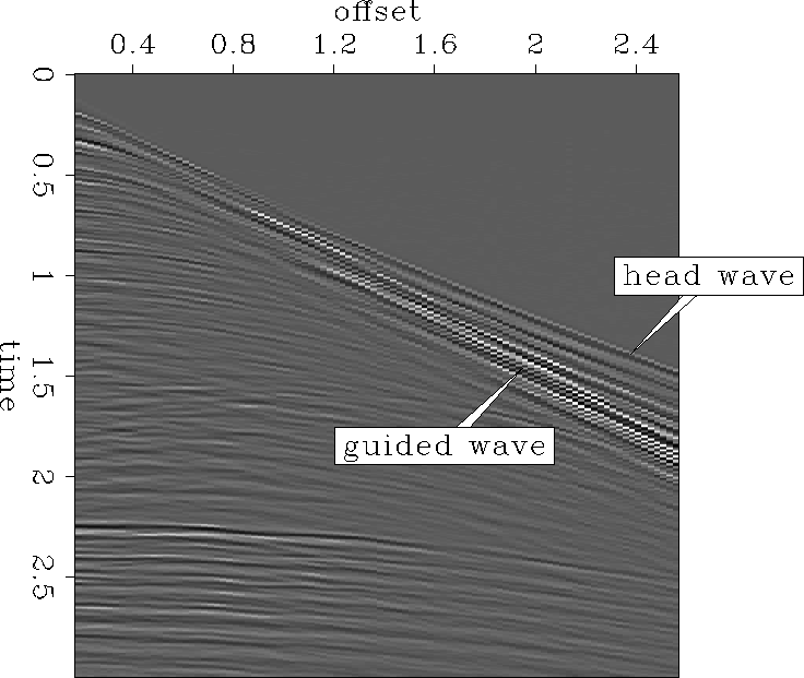
The data were recorded along parallel seismic lines as shown in Figure geo . The data I have are lines 115 to 132. The crossline spacing between the parallel seismic lines is 75 meters. Along the seismic line, the shot and hydrophone interval is 25 meters. There are 240 shot gathers along lines 115 to 132, and 96 geophones along the cable. The time sampling interval is 4 milliseconds. One shot gather is shown in Figure ashotgather to illustrate the prestack data.

 

geo
Figure 1 The Oseberg acquisition geometry of parallel seismic lines.

 

ashotgather
Figure 2 One shot gather recorded along line 125.

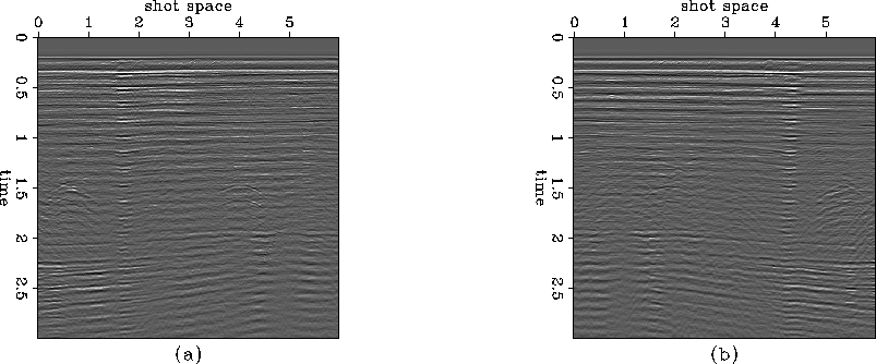
The lines were not consistently shot in the same direction. Lines 115 to 125 were shot in the opposite direction from lines 126 to 132, as shown in Figure nears. I took care to handle this when stacking. From these near-offset sections I can also see that the geological structure is quite flat, so it is reasonable to use a stacking velocity that only varies along the time axis.

 

nears
Figure 3 Near-offset sections show that line 125 is recorded in the opposite direction relative to line 126.
a. Near-offset section of line 125.
b. Near-offset section of line 126.

2-D stacking was performed on the data, one line at a time, by summing each NMO-corrected trace to its corresponding CMP bin. This method does not require sorting into CMP gathers. The CMP bin grid is overlaid on a real geological surface. The inline interval of the CMP bin grid is 12.5 meters. Since stacking for each line is done separately, the crossline interval of the CMP bin grid must be 75 meters.

I assumed that the stacking velocity was a function of time with the following form:

$$v(\tau) = v_0(\tau_0) + a*\tau^b \EQNLABEL{vstack}$$ (1)

Fig vrms shows the calculated rms velocity for stacking generated by Equation vstack using parameters a=0.5(km/s) and b=0.25.

 

vrms Figure 4 RMS velocity function used for brute stack.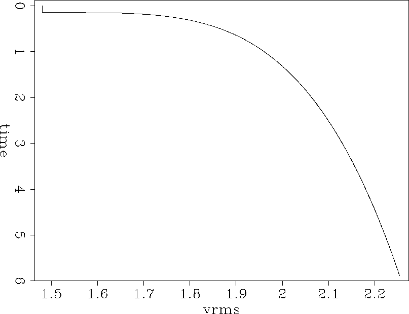

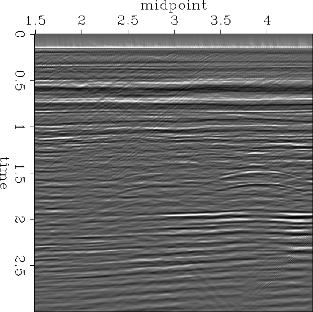
Figure stack shows the stacked section of line 125. Note the higher signal to noise ratio in comparison to Figure nears.

 

stack
Figure 5 The stacked section of line 125.

After stacking, the lines were merged to create a 3-D post-stack cube.

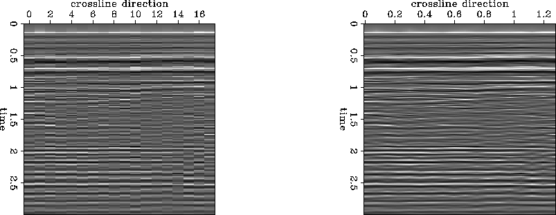
Since the geological structures do not change much in the cross line direction, I applied linear interpolation along the cross line to the stacked cube. The interpolated cube now has 12.5 meter interval in both the inline and the crossline direction. Figure interp shows the same slices along the cross line before and after interpolation. Linear interpolation seems justified due to the flat structure.

 

interp
Figure 6 Slices along the cross-line direction.
a. Before interpolation.
b. After interpolation.

MIGRATION

In order to test the difference between conventional two-pass depth migration and Ristow's four-pass depth migration on real data, both methods were applied to the stacked data.

When I did the two-pass and four-pass migration, I used the exploding-reflector concept (), so I only needed to concern myself with upward-coming waves.

When the velocity is slowly variable or independent of x and y, the conditions of full separation apply (). The dispersion relations for the two-pass and four-pass migration algorithm can be written like this:

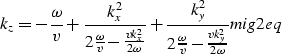$$k_z = -{\omega \over v} + \frac{k_x^2}{2{ \omega \over v}-{... ...\omega \over v}-{{vk_y^2} \over {2 \omega}}} \EQNLABEL{mig2eq}$$ (2)

$$k_z = {1 \over 2} {\left [-2{\omega \over v} + \frac{k_x^2}... ...er \sqrt{2}})^2} \over {2 \omega}}} \right ]} \EQNLABEL{mig4eq}$$ (3)

Using the splitting method, I can separate Equation mig2eq and Equation mig4eq into a retardation term and a diffraction term as follows:

$$\frac{\partial U}{\partial z}=-i{\omega \over v}U$$ (4)

two-pass:

$$\frac{\partial U}{\partial z}= {\left [\frac{ik_x^2}{2{ \om... ... v}-{{vk_y^2} \over {2 \omega}}} \right ]}U \EQNLABEL{diffr2}$$ (5)

four-pass:

$$\frac{\partial U}{\partial z}= {1 \over 2}{\left [\frac{ik_... ...v} -{{vk_y'^2} \over {2 \omega}}} \right ]}U \EQNLABEL{diffr4}$$ (6)

where k_x' and k_y' are the new axes after a rotation by 45 degrees:

$$k_x' = {k_x \over \sqrt{2}} + {k_y\over \sqrt{2}}$$ (7)

$$k_y' = -{k_x \over \sqrt{2}} + {k_y\over \sqrt{2}}$$ (8)

The counterpart of the diffraction equations in the ($\omega,x,y,z$) domain

$$\frac{\partial U}{\partial z }= {\left [\frac{-i \frac {\par... ...\frac{v \frac {\partial^2}{\partial y^2}}{2 \omega}} \right ]}U$$ (9)

$$\frac{\partial U}{\partial z }={1 \over 2} {\left [\frac{-i ... ...frac{v \frac {\partial^2}{\partial y'^2}}{2 \omega}} \right ]}U$$ (10)

is the equation I use to derive the differencing star and do migration.

To realize the four-pass method, I first apply the diffraction term along the x axis for all y and along the y axis for all x, just as in the two-pass method, except that I use dz / 2 to get the differencing star. I then sort the data along the x' axis and apply the diffraction term along x' for all y'. Next I sort the data along the y' axis and apply the diffraction term for all x'. Finally, the retardation term is applied, followed by imaging for each depth.

The migration codes are written in CM Fortran. The computing time is around three times faster than using Fortran 77 due to the parallel algorithm. I use Dave Hale's coding method for the zero slope boundary condition (Claerbout, 1985, Page 106) to take advantage of parallel computing.

Figure impulser shows the impulse response of the two migration operators. The four-pass operator is more isotropic than the two-pass one.

 

impulser
Figure 7 Comparison of the impulse responses of the two-pass and four-pass migration methods.
a. Depth slice from the two-pass technique.
b. Depth slice from the four-pass technique. It is more circular than that of the two-pass method.

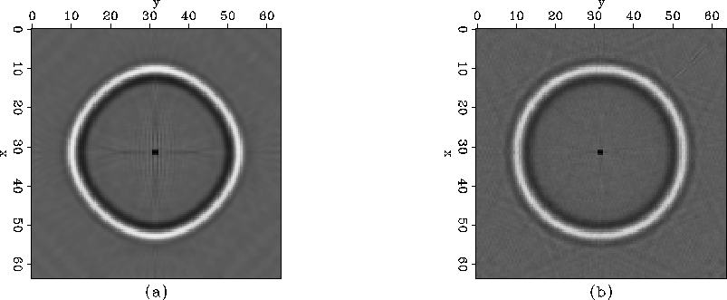Figure vmig shows the velocity function for migration. I calculated it from given RMS velocities at various depths.

 

vmig Figure 8 Migration velocity varies with depth.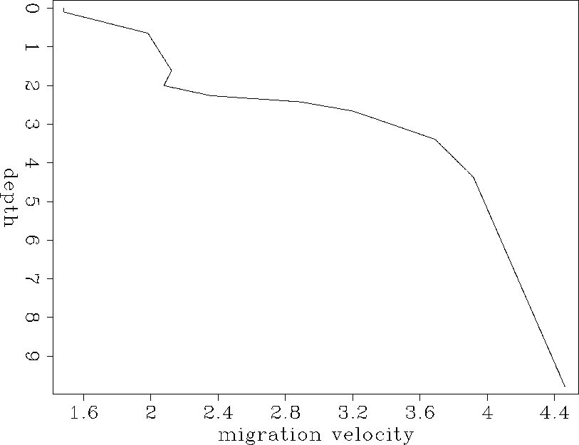

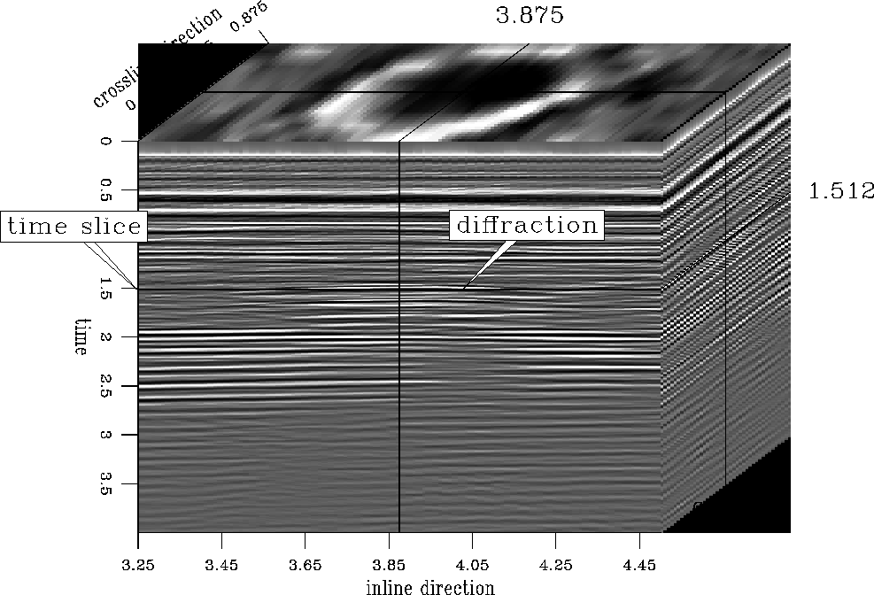
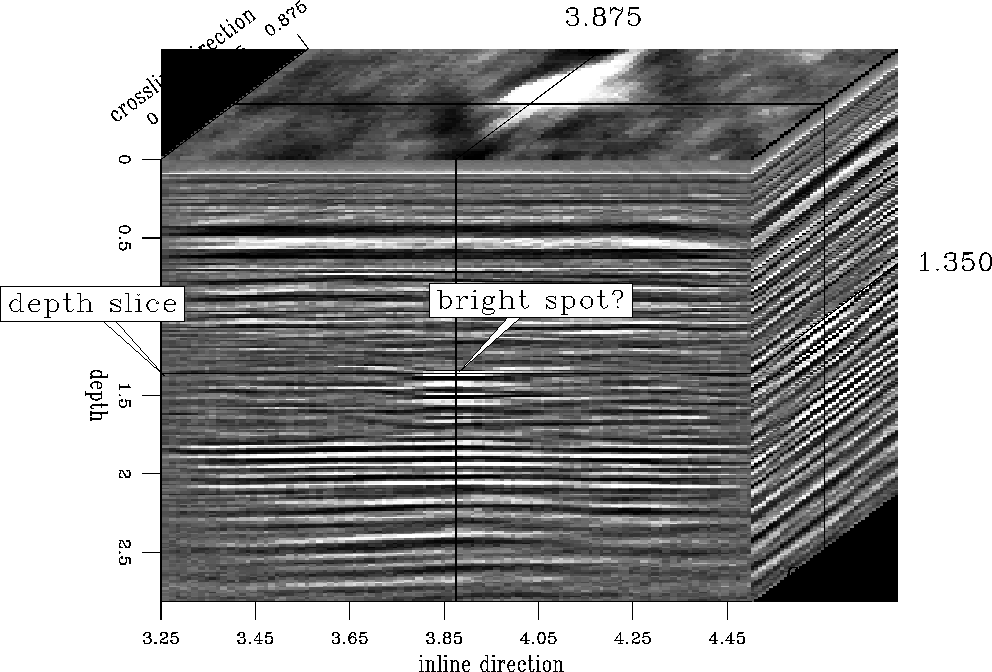
Figure apremigcube shows one stacked section before migration. The results after applying two-pass and four-pass migration, are displayed in Figure amig2cube and Figure amig4cube. The dip of the reflectors is very small. But it is obvious that the diffraction hyperbolas collapse after migration.

 

apremigcube
Figure 9 The stacked cube before migration.

 

amig2cube
Figure 10 Result of two-pass migration.

 

amig4cube
Figure 11 Result of four-pass migration.

DISCUSSION The difference between the two-pass and four-pass migration results on Oseberg data is not very obvious, although the impulse response shows that the four-pass migration operator is more isotropic than that of the two-pass. The first reason is that the data generated from brute stack and linear interpolation are coarse. Linear interpolation actually degrades the isotropy of a point source diffraction hyperbola. Second, velocity has lateral variation. Assuming that velocity just varies with depth is an approximation. Third, even the four-pass migration operator is not exact. Its error increases with the dip of the ray path.

ACKNOWLEDGMENTS I would like to thank David Lumley for helping me to learn some practical aspects of processing 3-D prestack data, and for lending me his computer codes and time to stack the Oseberg 3-D data. Hans Helle and Norsk Hydro kindly provided the Oseberg 3-D prestack data set to SEP, as arranged by David Lumley and Martin Karrenbach.

[fourpass]