Next: Migration velocity analysis
Up: Cole & Karrenbach: Least-squares
Previous: SOLVERS
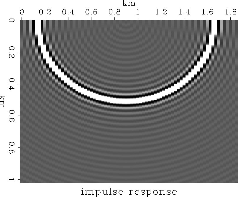
The impulse response of the migration algorithm is shown in
Figure ![[*]](http://sepwww.stanford.edu/latex2html/cross_ref_motif.gif) . To test the effect of a limited aperture,
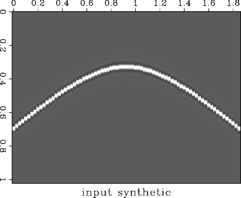
we generated a simple synthetic zero-offset section containing a
single hyperbolic event, as shown in Figure .
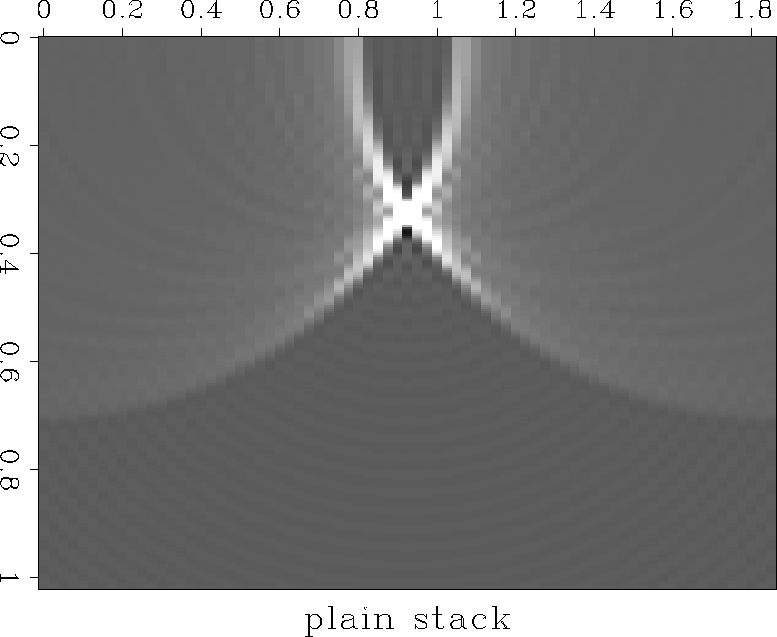
A conventional Kirchhoff migration, using all the traces, is
shown in Figure , and a migration where the
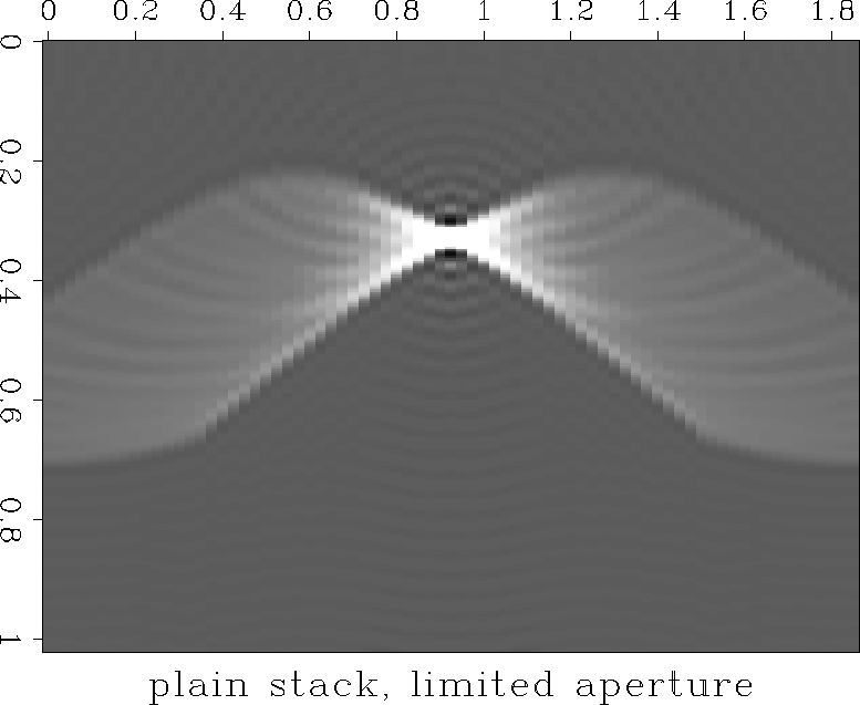
aperture is limited to the nearest 15 traces (the section
contains 75 traces) is shown in Figure .
The resolution in the limited aperture migration is not as good.
The same two plots are shown for the least-squares
case in Figures and . The limited
aperture result has improved resolution compared to the
non least-squares case.
impulse
. To test the effect of a limited aperture,
we generated a simple synthetic zero-offset section containing a
single hyperbolic event, as shown in Figure .
A conventional Kirchhoff migration, using all the traces, is
shown in Figure , and a migration where the
aperture is limited to the nearest 15 traces (the section
contains 75 traces) is shown in Figure .
The resolution in the limited aperture migration is not as good.
The same two plots are shown for the least-squares
case in Figures and . The limited
aperture result has improved resolution compared to the
non least-squares case.
impulse
Figure 3 Impulse response of migration
algorithm. This is a single slice from the 3D cube,
taken along the t=t0 plane.
 model
model
Figure 4 Synthetic dataset used to test the
migration scheme. Single point scatterer, constant velocity of 3 km/sec.
75 traces with a trace spacing of 25 meters.


 stack
stack
Figure 5 Conventional Kirchhoff migration of
synthetic dataset. Single slice from 3D cube at t=t0.
stacklim
Figure 6 Conventional Kirchhoff migration of
synthetic dataset, but migration aperture has been limited to
15 of 75 traces.
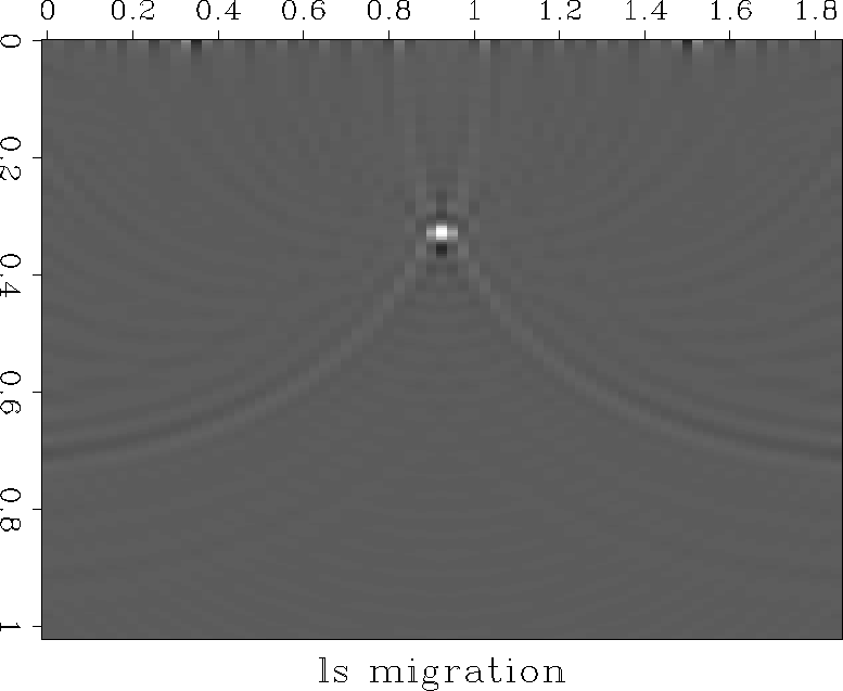
lsmig
Figure 7 Least-squares Kirchhoff migration.
Gives a better focus because effect of aperture has been removed.
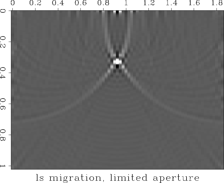
lsmiglim
Figure 8 Least-squares Kirchhoff migration,
aperture limited to 15 of 75 traces.
Some noise appears at the top of the least-squares
sections in Figures and .
These first few samples correspond to the
earliest t0 values (hyperbolas with the largest
amount of moveout). The noise
does not appear to be due to frequency-domain wraparound,
or aliasing,
and damping the least-squares method doesn't seem to help.
The noise is sufficiently strong, particularly away from
the single image plane shown in the figures, that it is
a cause for concern.
We hope to come up with a solution in the near future,
but weren't able to do so in time for this report.
This problem doesn't take away from the main result, as shown
in the figures, that the focusing of migration is less
affected by the limited aperture in the least-squares case.
The cost of this method is considerable. The conjugate
gradient algorithm runs for an average of about twenty
iterations on each frequency. This means multiplication
by the L or LH matrix an average of forty times,
versus a single multiplication for the non least-squares case.
The aperture compensation provided by least-squares must
be considerable if this method is to be worth the extra
cost. If least-squares allows us to migrate using fewer
traces, however, then the system of equations will be
smaller, and the extra cost will not be so large.
Another way to reduce the cost is to consider a target
oriented scheme, where only those hyperbola shapes appropriate
for the target zone are used for the third axis of the
migration cube. This would again make the least-squares
problems smaller, and reduce the cost.
Next: Migration velocity analysis
Up: Cole & Karrenbach: Least-squares
Previous: SOLVERS
Stanford Exploration Project
11/17/1997