The Haar Transform

The Haar transform is the simplest of the wavelet transforms. This transform cross-multiplies a function against the wavelet shown in Figure with various shifts and stretches, much like the Fourier transform cross-multiplies a function against a sine wave with two phases and many stretches.

 

haarplot Figure 7 The Haar wavelet.

As an example of a Haar transform, consider transforming the single seismic trace shown in Figure . The Haar transform of this trace is shown in Figure . Notice that the trace consists of two zones, a weak zone on the left side, and a strong zone on the right side. We see this pattern of strong and weak zones reflected as octave zones within the transform shown in Figure .

The samples in the Haar transform shown in Figure are coefficients that describe the decomposition of the trace in Figure . A simple example of the Haar decomposition is taken from Strang(1989). If f is a 4-sample trace, then

$$f = \pmatrix{ 9 \cr 1 \cr 2 \cr 0 \cr} = 3 \pmatrix{ 1 \... ...cr 0 \cr 0 \cr} +1 \pmatrix{ 0 \cr 0 \cr 1 \cr -1 \cr},$$ (1)

and the coefficients of the transform are $\pmatrix{3 \cr 2 \cr 4 \cr 1 \cr}$.

The first sample in Figure contains the coefficient that describes the D.C. component of the trace. The next sample contains the coefficient that describes how a single Haar wavelet shown in Figure cross-multiplies the entire trace. Then, the next two samples describe the two Haar wavelets that cross-multiply two-halves of the trace; one cross-multiplying the first half of the trace, the other cross-multiplying the last half of the trace. This halving of the wavelet and of the trace continues until the Haar wavelets are two samples long, and the number of coefficients required to describe the cross-multiplication are half the trace length. On the right side of Figure , in the last half of the trace, the amplitude pattern of the original trace is clearly reflected. This pattern may also be seen within the other octave zones.

 

trace Figure 8 A seismic trace with a low-energy zone and a high-energy zone.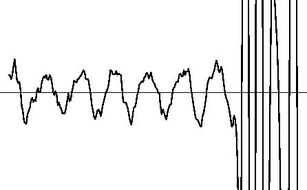

 

haartrace Figure 9 The Haar transform of the seismic trace shown in the previous figure.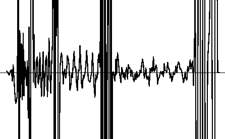

An alternate and perhaps more understandable method of displaying the results of a wavelet transform is in the two-dimensional display shown in Figure . The vertical axis is the time axis corresponding to the time axis of the trace. The horizontal axis corresponds to the sizes of the Haar wavelets. Where the longer operators have barely visible coefficients in Figure , Figure gives more emphasis to the long-operator coefficients and maintains the relative time scales within each set of coefficients.

 

dhaartrace Figure 10 The alternate display form of the Haar transform. The horizontal axis corresponds to the Haar wavelets sizes, and the vertical axis corresponds to the time axis of the trace. Notice that time increases vertically, opposite to the standard seismic display convention. This figure shows the same information as Figure 9.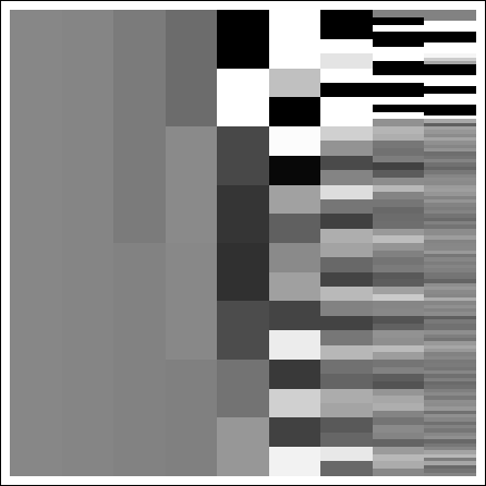

The algorithm is simple, however there is not an obvious use for the transformed data. The data is localized in time, but the frequency separation is poor when compared to the sliding Fourier transform.