References

• Cabrera, J., J., Perkins, W. T., Ratcliff, D. W., and Lynn, W., 1992, 3-D prestack depth migration on a massively parallel computer: implementation and case history: 54th Mtg. Eur. Assoc. Expl. Geophys., Abstracts, 268-269.

• Cervený, V., Molotkov, I. A., and Psencík, I., 1977, Ray method in seismology: Univerzita Karlova, Praha.

• Beydoun, W. B., and Keho, T. H., 1987, The paraxial ray method: Geophysics, 52, 1639-1653.

• Keho, T. H., and Beydoun, W. B., 1988, Paraxial ray Kirchhoff migration: Geophysics, 53, 1540-1546.

• Luo, Y., and Schuster, G. T., 1990, Wave-equation traveltime inversion: 60th Annual Internat. Mtg., Soc. Expl. Geophys., Expanded Abstracts, 1207-1210.

• Strang, G., 1980, Linear algebra and its applications: Academic Press.

• Van Trier, J., 1991, A massively parallel implementation of prestack Kirchhoff depth migration: 53rd Mtg. Eur. Assoc. Expl. Geophys., Abstracts.

• Van Trier, J., and Symes, W. W., 1991, Upwind finite-difference calculation of traveltimes: Geophysics, 56, 812-821.

• Vidale, J. E., 1988, Finite-difference calculation of traveltimes: Bull. Seis. Soc. Am., 78, 2062-2076.

• Zhang, L., 1992, Wavefront propagation by local ray-tracing: this report.

 

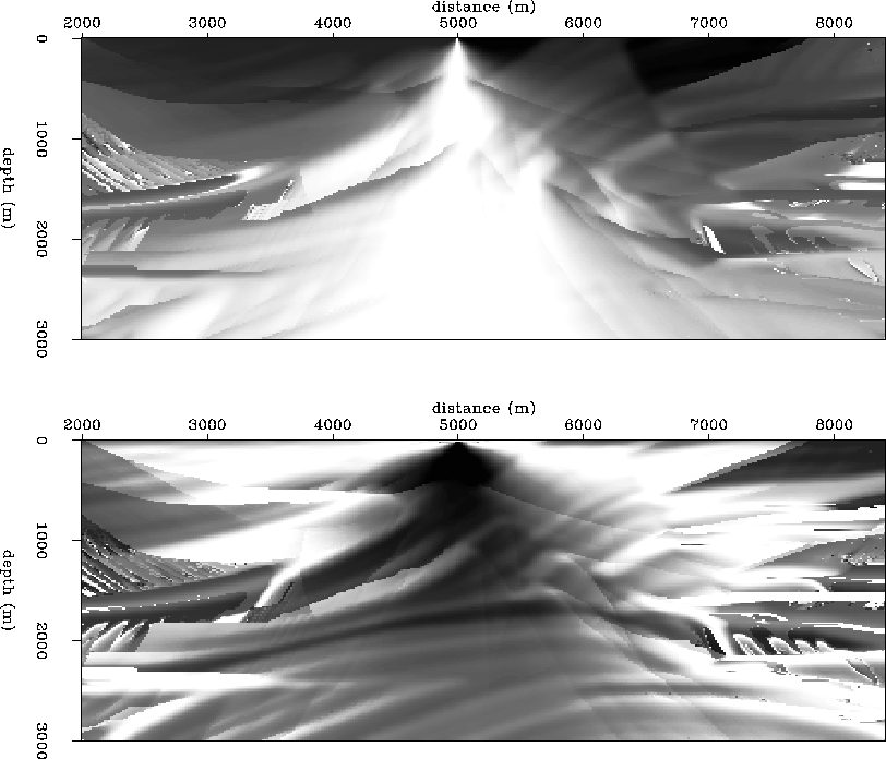
marmousi
Figure 12 Marmousi 2-D velocity model. Top panel is original velocity model, lower panel is a smoothed version using a pyramid of base half-width equal to 80 m, which is used for the traveltime and interpolation calculations.

 

m13t
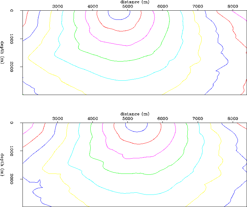
Figure 13 Marmousi velocity model. Contours of traveltime field for the two given surface source positions at 4.75 km (top) and 5.25 km (bottom).

 

m1xz
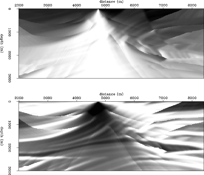
Figure 14 Marmousi velocity model. Horizontal (top) and vertical (bottom) traveltime gradient fields for the surface source positioned at 4.75 km.

 

m3xz
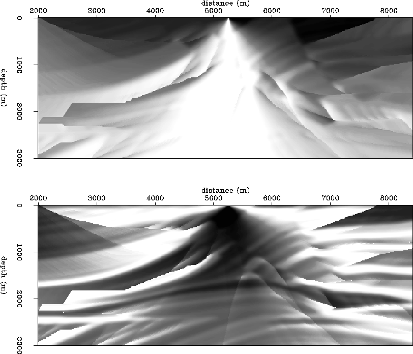
Figure 15 Marmousi velocity model. Horizontal (top) and vertical (bottom) traveltime gradient fields for the surface source positioned at 5.25 km.

 

mite
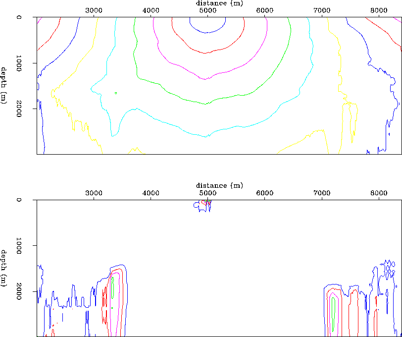
Figure 16 Marmousi velocity model. Interpolated traveltime field. The top panel is the interpolated traveltime field for a surface source positioned at 5.00 km. The lower panel is the relative error between the interpolated traveltime field, and the correct traveltimes modeled by finite differencing the eikonal. The contour farthest from the source region is at 5% relative error, and the contour values increase to 50% error right at the source location, in 5% contour increments.

 

mixz
Figure 17 Marmousi velocity model. Horizontal (top) and vertical (bottom) traveltime gradient fields for the interpolated surface source positioned at 5.00 km.