SYMMETRIZING THE WAVE FIELD

I am using the basic notion of symmetry in a wave field, or to be more precise the lack thereof. To expand that idea, let us look at a single slice through a prestack data volume. Let the data depend on the following variables:  

$$\bf\rm D({\bf x_r},{\bf x_s},\omega) = \bf\rm S({\bf x_s},\... ...rm R({\bf x_s},\omega) + \bf\rm N({\bf x_r},{\bf x_s},\omega) ,$$ (1)

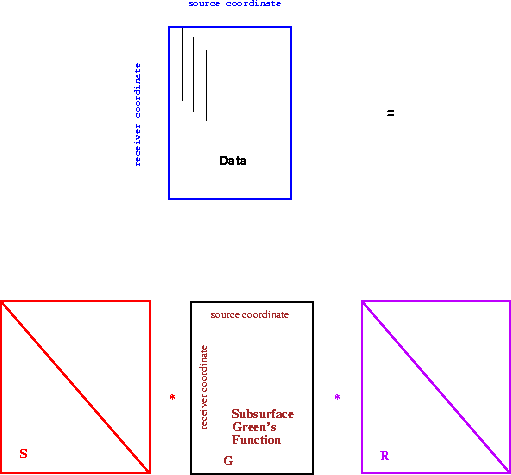
where $\bf\rm S$ describes the source behavior, $\bf\rm R$ describes the receiver behavior, and $\bf\rm G$ governs pure propagation effects through the medium. $\bf\rm N$ is an additive noise term. In an ideal world $\bf\rm N$ would be zero, as in Figure . $\bf\rm G$ represents the Green's function of the medium. It can be shown that since the anisotropic elastic wave equation is linear and self-adjoint, the discrete representation of the continuous function $\bf\rm D$ has to be symmetric. That is,  

$$\bf\rm S~\bf\rm G~\bf\rm R~=~(\bf\rm S~\bf\rm G~\bf\rm R)^T~=~ \bf\rm R^T~\bf\rm G^T~\bf\rm S^T .$$ (2)

This equation defines a measure for the symmetry of a given data set. The symmetric part of data is defined as

$$\bf\rm SYM = {{(\bf\rm S~\bf\rm G~\bf\rm R~+~\bf\rm R^T~\bf\rm G^T~\bf\rm S^T)}\over{2}}$$ (3)

and the antisymmetric part of the data as

$$\bf\rm DEV = {{( \bf\rm S~\bf\rm G~\bf\rm R~-~ \bf\rm R^T~\bf\rm G^T~\bf\rm S^T)}\over{2}} .$$ (4)

 

matrix
Figure 1 Schematic representation of a discrete symmetric wave field