

Next: Field data removing tube
Up: NUMERICAL EXAMPLES
Previous: NUMERICAL EXAMPLES
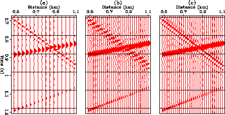
Figure ![[*]](http://sepwww.stanford.edu/latex2html/cross_ref_motif.gif) a shows
a synthetic section containing three linear events, each of which has
a different wavelet. The steepest event has a high-pass wavelet and is
almost completely aliased in space. The event with its amplitude decaying
along its trajectory has an all-pass wavelet. Finally, the flattest
event has a low-pass wavelet. Figure
a shows
a synthetic section containing three linear events, each of which has
a different wavelet. The steepest event has a high-pass wavelet and is
almost completely aliased in space. The event with its amplitude decaying
along its trajectory has an all-pass wavelet. Finally, the flattest
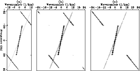
event has a low-pass wavelet. Figure ![[*]](http://sepwww.stanford.edu/latex2html/cross_ref_motif.gif) a shows the 2-D spectrum of
this section. Clearly, the dip structure in this example varies
with respect to frequencies. Figures
a shows the 2-D spectrum of
this section. Clearly, the dip structure in this example varies
with respect to frequencies. Figures ![[*]](http://sepwww.stanford.edu/latex2html/cross_ref_motif.gif) b and
b and ![[*]](http://sepwww.stanford.edu/latex2html/cross_ref_motif.gif) c
show the first-order
interpolation with Spitz's algorithm and our algorithm, respectively.
We can see that both algorithms correctly interpolate two gentle-dip events,
even though one of the events has amplitude variation. Spitz's formulation
does not explicitly consider the amplitude variations of events, but it is
valid when the amplitude variations do not depend on frequency;
frequency-dependent amplitude variations may cause some
minor problems.
Spitz's algorithm fails, however, to interpolate in the correct dip
direction of the steepest event that is completely aliased in space
because of the frequency-dependent dip structure of data. In contrast,
our algorithm interpolates the event correctly. Figures
c
show the first-order
interpolation with Spitz's algorithm and our algorithm, respectively.
We can see that both algorithms correctly interpolate two gentle-dip events,
even though one of the events has amplitude variation. Spitz's formulation
does not explicitly consider the amplitude variations of events, but it is
valid when the amplitude variations do not depend on frequency;
frequency-dependent amplitude variations may cause some
minor problems.
Spitz's algorithm fails, however, to interpolate in the correct dip
direction of the steepest event that is completely aliased in space
because of the frequency-dependent dip structure of data. In contrast,
our algorithm interpolates the event correctly. Figures ![[*]](http://sepwww.stanford.edu/latex2html/cross_ref_motif.gif) b
and
b
and ![[*]](http://sepwww.stanford.edu/latex2html/cross_ref_motif.gif) c show the 2-D spectra of the interpolated sections, which confirm
our observations in the time-space domain. Figure
c show the 2-D spectra of the interpolated sections, which confirm
our observations in the time-space domain. Figure ![[*]](http://sepwww.stanford.edu/latex2html/cross_ref_motif.gif) c also
displays, at frequency 40 Hz and wavenumber 8 (1/km), a gap in one event,
which is a noticeable pitfall
of our algorithm. This occurs because our zero-searching routine
assumes a single-zero presence at each location. Hence, the neural net may
reject a genuine zero if it coincides with a fake zero. Because
this problem occurs at only a few frequencies, we do not expect
it to have strong impact on the later processing of the interpolated
data.
c also
displays, at frequency 40 Hz and wavenumber 8 (1/km), a gap in one event,
which is a noticeable pitfall
of our algorithm. This occurs because our zero-searching routine
assumes a single-zero presence at each location. Hence, the neural net may
reject a genuine zero if it coincides with a fake zero. Because
this problem occurs at only a few frequencies, we do not expect
it to have strong impact on the later processing of the interpolated
data.
This synthetic example represents an extreme case that may or may not exist
in practice. However, it clearly reveals the important assumptions that
Spitz's algorithm entails.
syncom
Figure 4 A synthetic example of trace interpolation: (a) before interpolation,
(b) after interpolation with Spitz's algorithm,
(c) after interpolation with our algorithm.


 synspccom
Figure 5 Comparisons of 2-D spectra: (a) before interpolation,
(b) after interpolation with Spitz's algorithm,
(c) after interpolation with our algorithm.


Next: Field data removing tube
Up: NUMERICAL EXAMPLES
Previous: NUMERICAL EXAMPLES
Stanford Exploration Project
11/18/1997
![[*]](http://sepwww.stanford.edu/latex2html/cross_ref_motif.gif) a shows
a synthetic section containing three linear events, each of which has
a different wavelet. The steepest event has a high-pass wavelet and is
almost completely aliased in space. The event with its amplitude decaying
along its trajectory has an all-pass wavelet. Finally, the flattest
event has a low-pass wavelet. Figure
a shows
a synthetic section containing three linear events, each of which has
a different wavelet. The steepest event has a high-pass wavelet and is
almost completely aliased in space. The event with its amplitude decaying
along its trajectory has an all-pass wavelet. Finally, the flattest
event has a low-pass wavelet. Figure ![[*]](http://sepwww.stanford.edu/latex2html/cross_ref_motif.gif) a shows the 2-D spectrum of
this section. Clearly, the dip structure in this example varies
with respect to frequencies. Figures
a shows the 2-D spectrum of
this section. Clearly, the dip structure in this example varies
with respect to frequencies. Figures ![[*]](http://sepwww.stanford.edu/latex2html/cross_ref_motif.gif) b and
b and ![[*]](http://sepwww.stanford.edu/latex2html/cross_ref_motif.gif) c
show the first-order
interpolation with Spitz's algorithm and our algorithm, respectively.
We can see that both algorithms correctly interpolate two gentle-dip events,
even though one of the events has amplitude variation. Spitz's formulation
does not explicitly consider the amplitude variations of events, but it is
valid when the amplitude variations do not depend on frequency;
frequency-dependent amplitude variations may cause some
minor problems.
Spitz's algorithm fails, however, to interpolate in the correct dip
direction of the steepest event that is completely aliased in space
because of the frequency-dependent dip structure of data. In contrast,
our algorithm interpolates the event correctly. Figures
c
show the first-order
interpolation with Spitz's algorithm and our algorithm, respectively.
We can see that both algorithms correctly interpolate two gentle-dip events,
even though one of the events has amplitude variation. Spitz's formulation
does not explicitly consider the amplitude variations of events, but it is
valid when the amplitude variations do not depend on frequency;
frequency-dependent amplitude variations may cause some
minor problems.
Spitz's algorithm fails, however, to interpolate in the correct dip
direction of the steepest event that is completely aliased in space
because of the frequency-dependent dip structure of data. In contrast,
our algorithm interpolates the event correctly. Figures ![[*]](http://sepwww.stanford.edu/latex2html/cross_ref_motif.gif) b
and
b
and ![[*]](http://sepwww.stanford.edu/latex2html/cross_ref_motif.gif) c show the 2-D spectra of the interpolated sections, which confirm
our observations in the time-space domain. Figure
c show the 2-D spectra of the interpolated sections, which confirm
our observations in the time-space domain. Figure ![[*]](http://sepwww.stanford.edu/latex2html/cross_ref_motif.gif) c also
displays, at frequency 40 Hz and wavenumber 8 (1/km), a gap in one event,
which is a noticeable pitfall
of our algorithm. This occurs because our zero-searching routine
assumes a single-zero presence at each location. Hence, the neural net may
reject a genuine zero if it coincides with a fake zero. Because
this problem occurs at only a few frequencies, we do not expect
it to have strong impact on the later processing of the interpolated
data.
c also
displays, at frequency 40 Hz and wavenumber 8 (1/km), a gap in one event,
which is a noticeable pitfall
of our algorithm. This occurs because our zero-searching routine
assumes a single-zero presence at each location. Hence, the neural net may
reject a genuine zero if it coincides with a fake zero. Because
this problem occurs at only a few frequencies, we do not expect
it to have strong impact on the later processing of the interpolated
data.

