MODELING RESULTS

To test the accuracy of the proposed solution of the frequency-dependent eikonal equation I compared results obtained by extrapolating the phase slowness with the results obtained from a wave-equation modeling by finite differences. I used two simple models for this testing. Both models present a Gaussian-shaped circular velocity anomaly in a constant velocity background, in the first example the perturbation is negative, in the second one it is positive. I chose anomalies of opposite signs because I wanted to test the accuracy of my method both in presence of focusing of the wavefield (negative perturbation) and of defocusing (positive perturbation).

In the first example the background velocity is 3 km/s, the maximum amplitude of the anomaly is 1.5 km/s and its width is about 100 m. I started the extrapolation process at infinite frequency and stopped when it reached the frequency of 5 Hz. The extrapolation step was constant in inverse frequency $\phi$.Figure  shows a vertical slice of the resulting velocity model for three different frequencies. The solid line shows the medium slowness; that is, the infinite frequency slowness. The dashed line shows the phase slowness at 12.5 Hz, corresponding to a wavelength of 240 m. Finally the dotted line shows the phase slowness at 5 Hz, corresponding to a wavelength of 600 m. As frequency decreases, the frequency extrapolation progressively smooths the slowness model.

 

Velneg
Figure 1 A vertical slice of the phase-slowness function for three different frequencies: infinite frequency (solid line), 12 Hz (dashed line), and 5 Hz (dotted line).

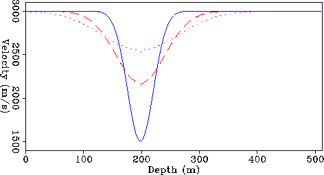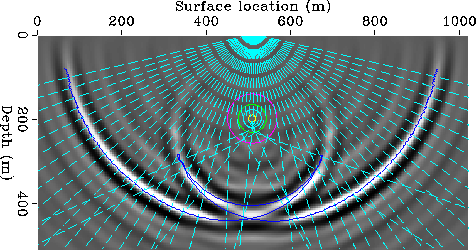
Figure  shows the results of wave-equation modeling and standard raytracing through the model. Plots of the rays (dashed lines) and the wavefront predicted by raytracing (solid black line) are superimposed onto a snapshot of the wavefield. The Figure also shows a contour plot of the velocity anomaly (white circles). For the wave-equation modeling I used a wavelet with central frequency of 60 Hz, corresponding to a wavelength of 50 m. This wavelength is sufficiently short, compared to the the width of the anomaly, for the eikonal to correctly predict the behavior of the wavefield. Just beneath the peak of the anomaly, the rays go through a caustic and the wavefront triplicates. The raytracing predicts correctly the positions and amplitudes of the different branches of the wavefield. 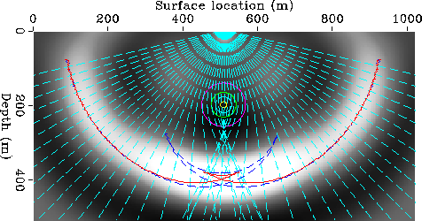In contrast, when the central frequency of the wavelet drops to 10 Hz (Figure ) the wavefront predicted by the eikonal does not match the actual wavefront of the wavefield. Figure  shows the result of wave-equation modeling with a 10 Hz wavelet and of raytracing through the extrapolated phase slowness at a frequency of 10 Hz. To facilitate the comparison, I actually plotted both the wavefront predicted by the phase slowness at 10 Hz (solid line) and the wavefront predicted by the medium slowness (dashed line). The low-frequency wavefront triplicates as well, but the inner branches are much shorter than the branches in the high-frequency wavefront. At the particular time of the snapshot, the low-frequency rays are still focused beneath the anomaly, consistently with the amplitudes of the actual wavefield, while the high frequency rays have already spread far apart.

 

Raynegvel60
Figure 2 A snapshot of the wavefield generated by a source with central frequency of 60 Hz after propagating through the negative anomaly. Plots of the velocity anomaly, the rays traced through the medium slowness, and the wavefront predicted by the rays are superimposed onto the wavefield.

 

Raynegvel10
Figure 3 A snapshot of the wavefield generated by a source with central frequency of 10 Hz after propagating through the negative anomaly. Plots of the velocity anomaly, the rays traced through the 10 Hz phase slowness, and the wavefronts predicted by the 10 Hz phase slowness (solid line) and by the medium slowness (dashed line) are superimposed onto the wavefield. (Compare with Figure )

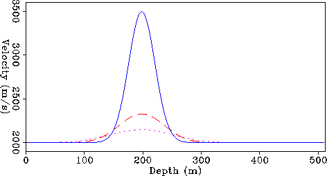
The second example is similar to the first, but the anomaly is positive instead of being negative, and thus the wavefield defocuses instead of focusing. The background velocity is 2 km/s, and the maximum amplitude of the anomaly is 1.5 km/s. I started the extrapolation process at infinite frequency, and stopped it when it reached 5 Hz. Figure  shows a vertical slice of the resulting velocity model for three different frequencies. The solid line in the Figure shows the medium slowness. The dashed line shows the phase slowness at 12.5 Hz, corresponding to a wavelength of 160 m. Finally the dotted line shows the phase slowness at 5 Hz, corresponding to a wavelength of 400 m. Also in this case the frequency extrapolation progressively smoothed the slowness function, but the respective scaling of the velocity perturbations are different from the previous example. In this case the 12.5 Hz anomaly has a peak of about $20\%$ the peak of the infinite frequency slowness, when in the previous case it was about $50\%$.This behavior is a clear indication that the smoothing is far from being linear in velocity. Although, the smoothing might be close to be linear in slowness; this issue deserves further study.

 

Velpos
Figure 4 A vertical slice of the phase-slowness function for three different frequencies: infinite frequency (solid line), 12 Hz (dashed line), and 5 Hz (dotted line). (Compare with Figure )

 

Rayposvel60
Figure 5 A snapshot of the wavefield generated by a source with central frequency of 60 Hz after propagating through the positive anomaly. Plots of the velocity anomaly, the rays traced through the medium slowness, and the wavefront predicted by the rays are superimposed onto the wavefield.

 

Rayposvel10
Figure 6 A snapshot of the wavefield generated by a source with central frequency of 10 Hz after propagating through the positive anomaly. Plots of the velocity anomaly, the rays traced through the 10 Hz phase slowness, and the wavefronts predicted by the 10 Hz phase slowness (solid line) and by the medium slowness (dashed line) are superimposed onto the wavefield. (Compare with Figure )

Figure  shows the results of wave-equation modeling with a 60 Hz wavelet and of raytracing through the medium slowness. The rays (dashed lines) and the wavefront predicted by raytracing (solid black line) are superimposed onto a snapshot of the wavefield. The wavefield is defocused by the anomaly; the anomaly causes a ``shadow zone'' beneath itself, where the amplitudes are very low. The high-frequency rays go through a caustic on either side of the anomaly, and thus the wavefront triplicates. The wavelength of the wavefield is too short (about 30 m) to observe wavefield dispersion and thus the raytracing through the medium slowness accurately predicts the behavior of the wavefield. In contrast, the low-frequency wavefield (Figure ) behaves quite differently from the high-frequency one. The wavefront does not triplicate and although the amplitudes beneath the anomaly are lower than on the side, they are not as low as in the high-frequency wavefield. The position of the wavefront and the amplitudes of the wavefield are well predicted by raytracing through the 10 Hz phase slowness computed using the frequency extrapolation method that I have presented. Beneath the anomaly, the distance between the wavefront predicted by the low-frequency phase slowness and the one predicted by the medium slowness is about 20 m; that is, the conventional eikonal would cause an error of about ${\pi \over 5}$in modeling the propagation of a 10 Hz wavefield through the anomaly.