Calculating the phase spectrum

The phase spectrum is usually calculated by taking the arctangent of the ratio of imaginary to real parts of the Fourier transform. Because the arctangent function is a multivalue function, its principal value has to be determined as being, for example, between $-\pi$ and $\pi$. However, the phase spectrum calculated from the principal-value range is not a continuous function. It does not satisfy equation (5). One way to solve this problem is to add appropriate multiples of $2\pi$ to the samples of the principal value. The appropriate multiple of $2\pi$ can be determined by assuming that the sampling interval is sufficiently small so that the discontinuities between adjacent samples of the phase spectrum correspond to $2\pi$ phase-wrap-around. If the phase spectrum varies rapidly, zero padding should be done in the time domain to ensure that there is a sufficiently small sampling interval in frequency.

 

swhfactm Figure 1 The top panel shows a synthetic, minimum phase wavelet delayed for 80 ms. The middle and bottom panels show the minimum phase and maximum phase parts of this wavelet, respectively. The vertical dashed lines indicate the picking positions. The fat, dashed curve superposed on the curve of the top panel is the signal reconstructed from two factorized parts.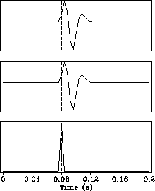

 

swhfactz Figure 2 The top panel shows a synthetic, zero phase wavelet delayed for 80 ms. The middle and bottom panels show the minimum phase and maximum phase parts of this wavelet, respectively. The vertical dashed lines indicate the picking positions. The fat, dashed curve superposed on the curve of the top panel is the signal reconstructed from two factorized parts.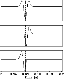

 

vwhfact Figure 3 The top panel shows a trace recorded in a marine survey. The middle and bottom panels show the minimum phase and maximum phase parts of this wavelet, respectively. The vertical dashed lines indicate the picking positions. The fat, dashed curve superposed on the curve of the top panel is the signal reconstructed from two factorized parts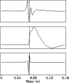

Now let us look at some examples. Figure shows a minimum wavelet with a delay of 0.08 second. After the spectrum factorization, the minimum phase part is the original wavelet and the maximum phase part is a spike. We see that the algorithm picks the first break. Figure shows the results in the case of a zero phase wavelet. As expected, the central peak of the zero phase wavelet is picked. In both cases, the correct delays are found. Figure shows the picking result of a trace recorded in a marine survey. The wavelet generated by an air-gun propagates through water and is recorded by a hydrophone. It is apparent that the picking position is not the first break. The minimum phase part contains mainly low frequency components while the maximum phase part contains only high frequency components. The non-overlapping spectra of two parts indicate that the factorization algorithm may become numerically unstable. However, the instability of the spectrum factorization does not affect the results of traveltime picking because the formula for calculating n₀ uses the total phase response. The spectrum factorization is only used to explain the principle of picking.