TOEPLITZ STRUCTURE

The elements in the matrix ${\bf R}$ are

$$r_{lk} = \sum_i e^{-j\omega_l t_i}e^{j\omega_k t_i} = \sum_i e^{j(\omega_k-\omega_l)t_i}.$$ (6)

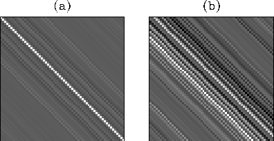
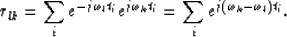
Because the frequency is uniformly sampled, $\omega_k-\omega_l$ is constant along diagonals of the matrix; hence the elements of the matrix ${\bf R}$ are also constant along its diagonals. Matrices with this kind of structure are called Toeplitz matrices. Since one can further show that symmetric elements with respect to the main diagonal of the matrix are complex conjugates, the matrix is Hermitian-Toeplitz. Figure shows an example of the real and imaginary parts of ${\bf R}$. With a left-side Hermitian-Toeplitz matrix, equation (5) can be efficiently solved using the generalized Levinson recursion (Golub and Van Loan, 1989; Kostov, 1989). The number of operations required is 2K², just twice the cost of multiplying a vector by a matrix. Once the discrete Fourier spectra are found, equation (2) can be used to evaluate the continuous signal s(t) at arbitrary positions. If the evaluations desired are at uniformly spaced positions, the fast Fourier transform should be used. When the input signal is uniformly sampled, matrix ${\bf R}$ becomes an identity matrix, and the whole interpolation process is equivalent to the ordinary sinc interpolation.

The elements of matrix ${\bf R}$ depend only on the sampling positions, not on the values of samples. Therefore, to interpolate missing traces, one can pre-compute the inverse of matrix ${\bf R}$, and then apply it to each time or frequency slice.

 

ata
Figure 1 Elements in the matrix ${\bf R}$ of a general normal equation set: (a) real part, (b) imaginary part.