

Next: CONCLUSIONS
Up: EXAMPLES
Previous: Traveltimes and rays
The amplitude calculation requires that the slowness models are smooth.
I apply the algorithm to compute the amplitudes for a medium having
a velocity function that increases linearly with depth. The velocity gradient is
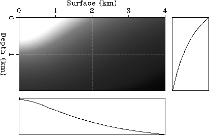
1.5 1/sec. Figure ![[*]](http://sepwww.stanford.edu/latex2html/cross_ref_motif.gif) shows the amplitudes computed
for a line source having an isotropic radiation pattern. The computed amplitudes
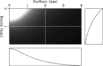
for a point source having an isotropic radiation pattern are shown in
Figure
shows the amplitudes computed
for a line source having an isotropic radiation pattern. The computed amplitudes
for a point source having an isotropic radiation pattern are shown in
Figure ![[*]](http://sepwww.stanford.edu/latex2html/cross_ref_motif.gif) . Comparing these two figures, we see that
for a point source, the amplitudes decay faster than for a line source.
Both figures show that large errors appear in a narrow region just below
the source position. These errors are due to the approximation of using
constant velocity cells in polar coordinates. To solve this problem,
I have proposed a new approach called the
local paraxial ray method (Zhang, 1991).
I expect
that the local paraxial ray method can handle the amplitude calculation
for slowness models containing reasonably large contrasts.
. Comparing these two figures, we see that
for a point source, the amplitudes decay faster than for a line source.
Both figures show that large errors appear in a narrow region just below
the source position. These errors are due to the approximation of using
constant velocity cells in polar coordinates. To solve this problem,
I have proposed a new approach called the
local paraxial ray method (Zhang, 1991).
I expect
that the local paraxial ray method can handle the amplitude calculation
for slowness models containing reasonably large contrasts.
ampgrals
Figure 5 Amplitudes for a model with a velocity function that is
linearly increasing as a function of depth.
The source is a line source with an isotropic radiation pattern,
located at the origin. The right and bottom panels show
cross sections of the amplitudes as functions of
depth and horizontal distance, respectively. The dashed lines indicate
the positions of the two cross sections.


 ampgraps
Figure 6 Amplitudes for a model with a velocity function that is
linearly increasing as a function of depth.
The source is a point source with an isotropic radiation pattern,
located at the origin. The right and bottom panels show
cross sections of the amplitudes as functions of
depth and horizontal distance, respectively. The dashed lines indicate
the positions of the two cross sections.


Next: CONCLUSIONS
Up: EXAMPLES
Previous: Traveltimes and rays
Stanford Exploration Project
12/18/1997
![[*]](http://sepwww.stanford.edu/latex2html/cross_ref_motif.gif) shows the amplitudes computed
for a line source having an isotropic radiation pattern. The computed amplitudes
for a point source having an isotropic radiation pattern are shown in
Figure
shows the amplitudes computed
for a line source having an isotropic radiation pattern. The computed amplitudes
for a point source having an isotropic radiation pattern are shown in
Figure ![[*]](http://sepwww.stanford.edu/latex2html/cross_ref_motif.gif) . Comparing these two figures, we see that
for a point source, the amplitudes decay faster than for a line source.
Both figures show that large errors appear in a narrow region just below
the source position. These errors are due to the approximation of using
constant velocity cells in polar coordinates. To solve this problem,
I have proposed a new approach called the
local paraxial ray method (Zhang, 1991).
I expect
that the local paraxial ray method can handle the amplitude calculation
for slowness models containing reasonably large contrasts.
. Comparing these two figures, we see that
for a point source, the amplitudes decay faster than for a line source.
Both figures show that large errors appear in a narrow region just below
the source position. These errors are due to the approximation of using
constant velocity cells in polar coordinates. To solve this problem,
I have proposed a new approach called the
local paraxial ray method (Zhang, 1991).
I expect
that the local paraxial ray method can handle the amplitude calculation
for slowness models containing reasonably large contrasts.

