

Next: CONCLUSION
Up: Ji: Trace Interpolation
Previous: RELATION TO CLAERBOUT'S AND
To compare the proposed interpolation scheme with Spitz`s method,
I applied the scheme to a data set which was similar to that
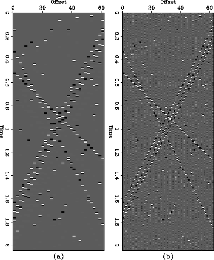
used by Spitz (1991, Spitz). Figure 2 shows synthetic data which
is spatially aliased linear events with random noises, and the result of
first-order interpolation. The result is comparable to that of Spitz.
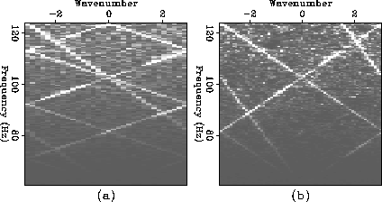
Figure 3 shows the spectra of data before and after interpolation.
The spectrum after interpolation fits well to our guess which
can be intuitively conjectured from the original spectrum.
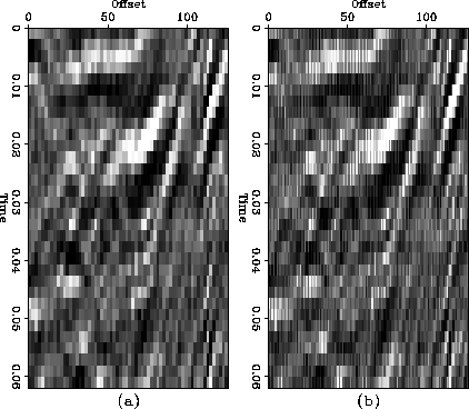
For a more realistic test, I have applied the interpolation scheme to a
real dataset which has aliased events.
The dataset, a 24-fold CMP stack of NMO-corrected Western offshore
Texas data, has been windowed to provide a smaller test dataset.
Figure 4 illustrates the performance of the interpolation scheme
proposed. It shows that the proposed algorithm may accommodate curvatures
and lateral amplitude variation.
fig2
Figure 2 (a)Input data made of three
aliased linear events (b) First order interpolated data. Note that
the parallel events have been correctly interpolated.
 fig3
fig3
Figure 3 Amplitude f-k spectra. The horizontal axes represent normalized wavenumber, from -0.5 to 0.5 cycles. (a)f-k
amplitude spectrum of the input shown in Figure 2(a). The unit scale of the normalized wavenumber is 1/32 cycles. (b) f-k amplitude spectrum of the interpolated data set shown in Figure 2(b). The unit scale of the normalized wavenumber is 1/64 cycles.
 fig4
fig4
Figure 4 (a)Input data which has windowed
from a CMP stack. (b) First order interpolated data.


Next: CONCLUSION
Up: Ji: Trace Interpolation
Previous: RELATION TO CLAERBOUT'S AND
Stanford Exploration Project
12/18/1997


