PROGRAMS

Subroutine tothin() copies the nonzero elements of a two-dimensional array bb(n1,n2) to a one-dimensional array b(), simultaneously determining it to be of size nb and making the two integer-valued subscription arrays b1(nb) and b2(nb).

# Copy 2-D array into a "thin" 1-D array by omitting zero values.
#
subroutine tothin( n1,n2,bb,   b1,b2,nb,b)
integer      i1,i2,n1,n2,      nb, b1(nb),b2(nb)
real         bb(n1,n2),        b(nb)
nb = 0
do i2= 1, n2 {
do i1= 1, n1 {
	if( bb(i1,i2) != 0.0 ) { nb = nb+1
		b1( nb) = i1
		b2( nb) = i2
		b ( nb) = bb(i1,i2)
		}
	}}
return;	end

Subroutine xthin() does crosscorrelation and convolution (conjugate pairs) of the ``thin'' arrays created by tothin(). The huge number of arguments arises because instead of characterizing a two-dimensional array as bb(n1,n2), we now characterize that two-dimensional array by b(nb),b1(nb),b2(nb),bm1,bm2 where two new integer parameters bm1 and bm2 define the origin or middle of the array. Given some familiarity with the coding style in PVI, the coding is easy especially since we merely abandon those points that fly beyond the edges of the array.

# Crosscorrelate 2-D thin filters  ('m' denotes midpoint)
#
subroutine xthin(conj,bm1,bm2,b1,b2,nb,b,am1,am2,a1,a2,na,a,cm1,cm2,n1,n2,cc)
integer bm1,bm2, ib,nb, b1(nb),b2(nb), ib1,ib2, conj
integer am1,am2, ia,na, a1(na),a2(na), ia1,ia2
integer cm1,cm2,     n1,    n2	     , ic1,ic2
real b(nb), a(na), cc(n1,n2)
call conjzero( conj, 0,  na, a,  n1*n2, cc)	# erase output
do ib= 1, nb { ib1 = b1(ib);	ib2 = b2(ib)
do ia= 1, na { ia1 = a1(ia);	ia2 = a2(ia)
	ic1 = cm1 + ib1-bm1 - (ia1-am1)		# Think of these lines as
	ic2 = cm2 + ib2-bm2 - (ia2-am2)		# (ic-cm) = (ib-bm) - (ia-am)
	if( ic1 > 0  &  ic1 <= n1)
	if( ic2 > 0  &  ic2 <= n2)		# Outputs on the mesh?
		if( conj == 0 )
			cc(ic1,ic2) = cc(ic1,ic2) + a(   ia   ) * b( ib)
		else
			a(  ia    ) = a(   ia   ) + cc(ic1,ic2) * b( ib)
	}}
return;	end

The least-squares simultaneous equation solution by conjugate gradients also follows the familiar pattern of PVI.

#	least squares fitting of thin kirchoff operator
#
subroutine lskirch(bm1,bm2,b1,b2,nb,b,am1,am2,a1,a2,na,a,rm1,rm2,n1,n2,rr,nitr)
integer bm1,bm2, nb, b1(nb),b2(nb), iter, nitr
integer am1,am2, na, a1(na),a2(na)
integer rm1,rm2,     n1,    n2	    
real b(nb), a(na), rr(n1,n2)
temporary real	dr(n1,n2), sr(n1,n2)
temporary real	da(na   ), sa(na   )
call zero( n1*n2, rr);			rr( rm1, rm2) = 1.0
call zero( na, a)
do iter= 0, nitr {
	call xthin(1,bm1,bm2,b1,b2,nb,b, am1,am2,a1,a2,na,da, rm1,rm2,n1,n2,rr)
	call xthin(0,bm1,bm2,b1,b2,nb,b, am1,am2,a1,a2,na,da, rm1,rm2,n1,n2,dr)
	call cgstep( iter, na,a,da,sa,  n1*n2,rr,dr,sr)
	}
return; end

After some experimentation I decided to incorporate the possibility of weighting functions. Defining a weighting function requires three more lines of code and applying it in the conjugate gradient code requires another three calls to a vector scaling subroutine. I named the vector scaling vscale() and the weighted least-squares fitting subroutine wlskirch().

#	c() = scale * a() * b()
#
subroutine vscale( scale, n, a, b, c )
integer i, n
real	scale, a(n), b(n), c(n)
do i= 1, n
	c(i) = scale * a(i) * b(i)
return;  end

wlskirch() which is littered with debugging snapshots.

#	Find WEIGHTED least squares inverse of thin kirchoff-type operator
#
subroutine wlskirch(bm1,bm2,b1,b2,nb,b,am1,am2,a1,a2,na,a,rm1,rm2,n1,n2,rr,ntr)
integer bm1,bm2, nb, b1(nb),b2(nb), iter, ntr
integer am1,am2, na, a1(na),a2(na)
integer rm1,rm2,     n1,    n2,		i1,i2, i
real	b(nb), a(na), rr(n1,n2),	dot, value
temporary real	dr(n1,n2), sr(n1,n2),   ww(n1,n2), wr(n1,n2)
temporary real	da(na   ), sa(na   )
temporary real	seea(n1,n2), seec(n1,n2)
call zero( n1*n2, rr);
		rr( rm1, rm2) = 1.0
do i1= 1, n1 {
do i2= 1, n2 {	ww(i1,i2) = sqrt( 1. + iabs(i1-rm1)  + iabs(i2-rm2) )
		}}
call vscale( 1., n1*n2, ww, rr, wr)
call zero( na, a)
do iter= 0, ntr {
	call vscale( 1., n1*n2, ww, wr, dr)
	call xthin(1,bm1,bm2,b1,b2,nb,b, am1,am2,a1,a2,na,da, rm1,rm2,n1,n2,dr)
	call xthin(0,bm1,bm2,b1,b2,nb,b, am1,am2,a1,a2,na,da, rm1,rm2,n1,n2,dr)
	call vscale( 1., n1*n2, ww, dr, dr)
	call cgstep( iter, na,a,da,sa,  n1*n2,wr,dr,sr)
######### begin diagnostic output
   if( iter <5 | iter==10 | iter==20 | iter==40 | iter == 80 ){
	value = dot( n1*n2, wr, wr)
	write(7,77) iter, value
	77 format( i3, f15.9)
        call zero( n1*n2, seea)
        do i= 1, nb
                seea( b1(i), b2(i) ) = a(i)
                                                call snap('aa.H', n1,n2, seea)
        call xthin( 0,  bm1,bm2, b1,b2,nb,b,
                        am1,am2, a1,a2,na,a,
                        rm1,rm2, n1,n2,  seec)
                                                call snap('cc.H', n1,n2, seec)
        }
        ######### end diagnostic output
	}
return; end

As ever, the main program is a bit of a clutter, though this one less so because the output is all being done from inside the subroutine. I tried to include the cakefile but L^ATEX insisted on looking for a file named cakefile.tex.

 

k0 Figure 1 Left is the ``Kirchhoff impulse response.'' Left is also the zero-th iteration of the estimated ``time-reversed inverse Kirchhoff impulse response'' or for short, ``Kirchhoff inverse.'' Right is the convolution of the two, i.e. the smear function of Kirchhoff modeling and migration.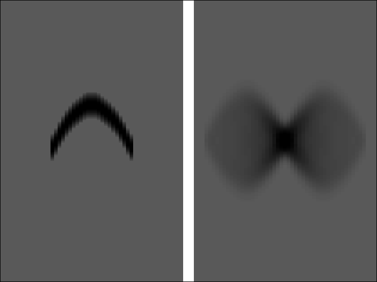

 

k8 Figure 2 Left is the 80-th iteration of the estimated Kirchhoff inverse. Right is the smear function. Push button for movie over iterations.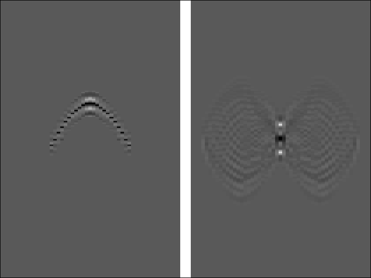

 

k1 Figure 3 Left is the first iteration of the estimated Kirchhoff inverse. Right is the smear function.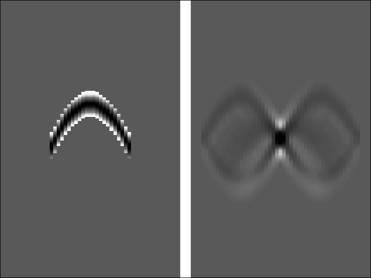

 

k5 Figure 4 Left is the tenth iteration of the estimated Kirchhoff inverse. Right is the smear function.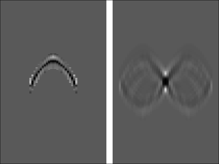