|
|
|
|
Efficient depth extrapolation of waves in elastic isotropic media |
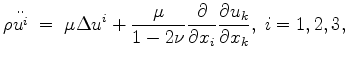
We start with the wave equation governing the displacement in an arbitrary heterogenous isotropic elastic medium in the Navier form (see (Segall, 2010)):
 denote the components of a displacement field,
  is the shear modulus,
  is Poisson's ratio for the medium, and
  is the density. In this paper we consider a heterogenous elastic medium under the assumption of local homogeneity - otherwise the elastic moduli would not be factored outside of the differentiation operators in equation 1. However, our method can be extended to cover the case when the local homogeneity assumption is dropped. ``Freezing'' the coefficients of equation 1 and applying the Fourier transform in time and horizontal variables
 , and substituting
 is the Lamé coefficient (see (Mavko et al., 2009),(Segall, 2010)), we get
 are horizontal wave numbers and
  is the frequency. The left-hand side of system 3 is the result of an ordinary differential operator applied to a vector-function
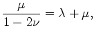
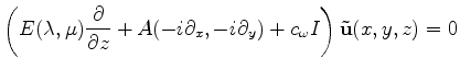
 and parameterized by horizontal wave numbers. In the present form equations 3 cannot be used for computationally efficient explicit depth extrapolation in a heterogeneous medium; however, these equations can be used for modeling displacements by solving a series of boundary-value problems (see (Maharramov, 2012)). In (Maharramov, 2012) it was suggested that equations 3 might be factorized in such a way as to allow solving them by alternating one-way extrapolation in opposite directions. More specifically, we seek a factorization of operator equation 3 of the form:
 |
![$\displaystyle = \;\left[ \begin{array}{ccc} \sqrt{\mu} & 0 & 0 \\ 0 & \sqrt{\mu} & 0 \\ 0 & 0 & \sqrt{\lambda+2\mu} \end{array} \right],$](img27.png) |
|
 |
 |
(5) |
 are
are  matrices with components that are complex-valued functions of the horizontal wave numbers,
  is the
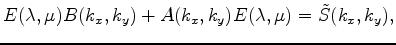
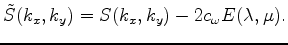
identity matrix. Performing the multiplication in equation 4 and using equation 3, we obtain:
is the
identity matrix. Performing the multiplication in equation 4 and using equation 3, we obtain:
 and
and  :
, for each pair of horizontal wave numbers
and two reference values of each elastic parameter
:
, for each pair of horizontal wave numbers
and two reference values of each elastic parameter
 and
and
 ;
;
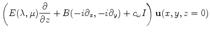
from the initial conditions and assign the value to an auxiliary function
 ;
;
 as e.g. in the PSPI method (see (Biondi, 2005)).
 by upward extrapolation:
 , however, it would reduce the cost of extrapolation by a further factor of 2. Note the cost of solving equation 10 in depth is roughly three times that of solving the scalar square-root equation.
The above analysis may be extended to the case of an arbitrary anisotropic elastic medium. The fact that the components of the pseudo-differential operator matrices
 are not given in an analytical form, but are only computed numerically, does not limit their applicability.
Factorization of system 3 in the elastostatic case was one of the approaches mentioned by the author in Maharramov (2012). However, the one-way extrapolation technique is mostly useful for elastodynamic problems as the passband of the factorized depth extrapolators (e.g., as in equation 11) narrows down to zero with the temporal frequency passing to the zero static limit.
|
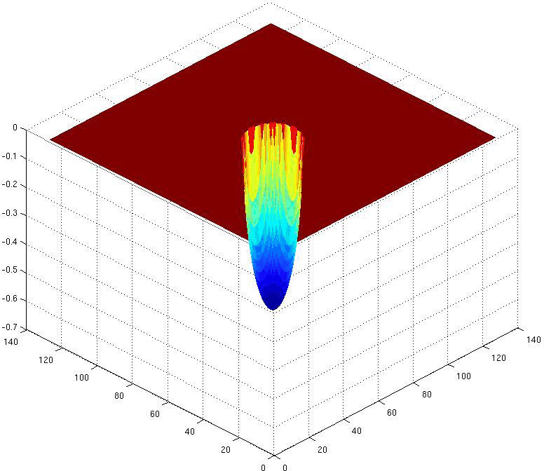
maximageigenval
Figure 1. The phase of a phase-shift operator corresponding to the maximum imaginary part of the eigenvalues of operator 15. Multicomponent ``phase-shift'' is defined by three such scalar phase-shift operators and a
matrix  of equation 16.
|
|
|---|---|
|
|
Note that equation 1 uses elastic parameterization that degenerates into a singularity if the shear modulus is equal to zero. This is not causing any problems with purely acoustic wave extrapolation as the singularity is effectively removed from equations 3 by the substitution in equation 2.
|
|
|
|
Efficient depth extrapolation of waves in elastic isotropic media |
![$\displaystyle \rho \omega^2 u^1+\mu\left[ (-k_x^2-k_y^2)u^1+\frac{\partial^2 u^...
...+\mu)\left[ -k_x^2 u^1-k_x k_y u^2+ik_x\frac{\partial u^3}{\partial z}\right] =$](img18.png)

![$\displaystyle \rho \omega^2 u^2+\mu\left[ (-k_x^2-k_y^2)u^2+\frac{\partial^2 u^...
...+\mu)\left[ -k_x k_y u^1-k_y^2 u^2+ik_y\frac{\partial u^3}{\partial z}\right] =$](img20.png)
![$\displaystyle \rho \omega^2 u^3+\mu\left[ (-k_x^2-k_y^2)u^3+\frac{\partial^2 u^...
... \frac{\partial u^2}{\partial z} + \frac{\partial^2 u^3}{\partial z^2}\right] =$](img21.png)
![$\displaystyle A(k_x,k_y)B(k_x,k_y)+c_{\omega}[A(k_x,k_y)+B(k_x,k_y)]$](img32.png)


![$\displaystyle \left[ \begin{array}{ccc} -(\lambda+2\mu)k_x^2 - \mu k_y^2 & -(\l...
...+2\mu)k_y^2 - \mu k_x^2 & 0 \\ 0 & 0 & -\mu(k_x^2 + k_y^2) \end{array} \right],$](img37.png)

![$\displaystyle \left[ \begin{array}{ccc} 0 & 0 & i (\lambda+\mu) k_x \\ 0 & 0 & ...
...da+\mu) k_y \\ i(\lambda+\mu) k_x & i(\lambda+\mu) k_y & 0 \end{array} \right].$](img39.png)

![$\displaystyle \tilde{u}(x,y,z+\Delta z)=\exp{\left[ -\Delta z E^{-1}(A(-i\partial_x,-i \partial_y)+c_{\omega}I)\right]}\mathbf{\tilde{u}}(x,y,z).$](img50.png)