 |
 |
 |
 | FWI with different boundary conditions |  |
![[pdf]](icons/pdf.png) |
Next: Gradient comparison
Up: Shen and Clapp: Boundary
Previous: Introduction
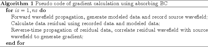
FWI as used here is a gradient-based time domain implementation (Shen, 2010). Different boundary conditions are used for the gradient calculation, leading to slight modifications of the gradient calculation algorithm. However, the steplength search uses absorbing boundary conditions in all cases.
The pseudo-code of the gradient calculation using the absorbing boundary condition is as follows:
The pseudo-code of the gradient calculation using the time-reversible boundary condition (random boundary condition and continuation of velocity) is as follows:
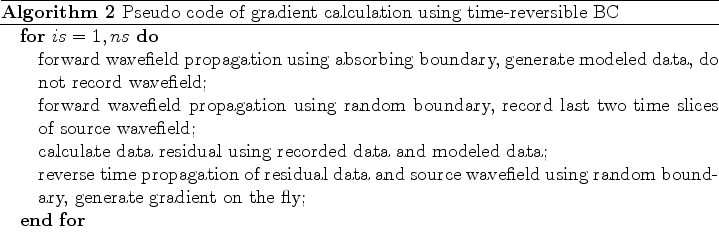
It is worth mentioning that for the MPI version of the code, wavefield propagation on different computational nodes uses different random boundary realizations, which further reduces artifacts.
2012-05-10