Early-arrival waveform inversion for near-surface velocity and anisotropic parameters: inversion of synthetic data

Complex synthetic

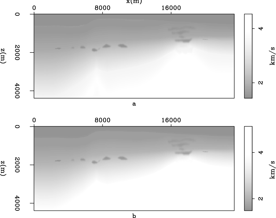
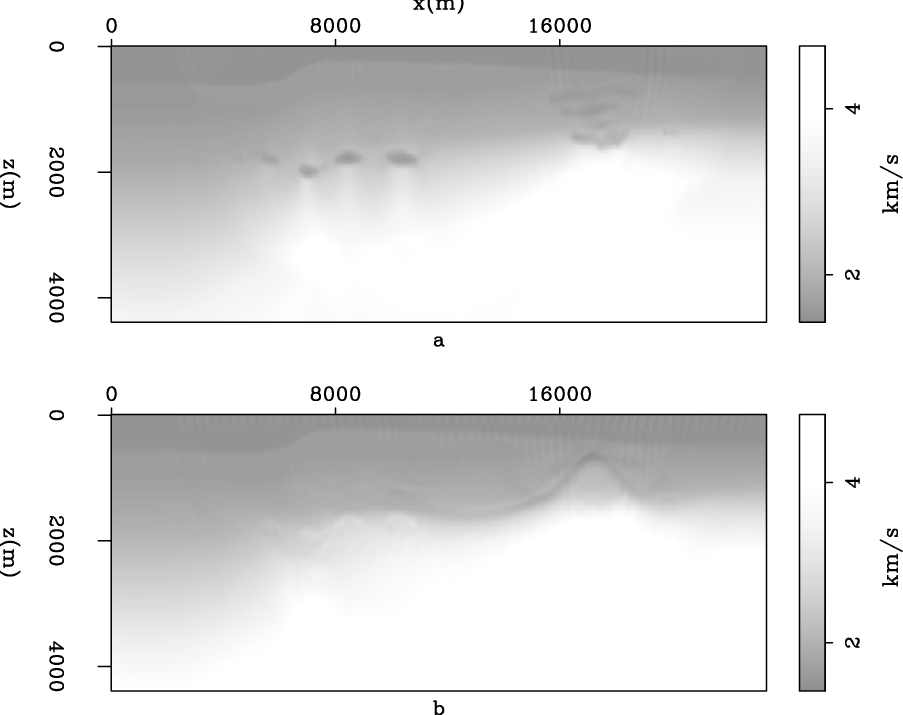
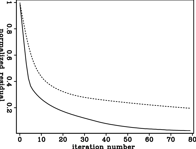
In this example, I invert the synthetic model shown in Figure 5. For joint inversion, starting models of vertical velocity and $\epsilon$ are a smoothed version of the true models without the shallow gas-pockets (Figure 6), and the $\delta$ parameter is fixed at zero. A total of $64$ shots with $320$ -m shot spacing are used, with sources of $7$ Hz peak frequency. The gas pocket sizes range from several hundred meters to almost two thousand meters. Given the dominant wavelength of the source wavelet, gas pocket sizes are on the order of several wavelengths, ensuring that most of the data misfit comes from the diving-wave traveltime difference. For simplicity, we assume that receivers are everywhere on the sea surface. The true model produces both refraction and reflection data. However, data masks are used during inversion to make sure that the inversion relies only on matching early arrivals that precede direct arrivals. Joint inversion results are shown for velocity parametrization in Figure 7, and for the logarithmic slowness parametrization in Figure 8. The logarithmic slowness parametrization yields a far superior model compared to inversion using velocity parametrization. This can also be seen in the data misfit comparison (Figure 9).

modelbw2
Figure 5. True model. a): velocity model; b): $\epsilon$ model.

initmodbw
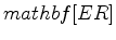
Figure 6. Starting model. a): velocity model; b): $\epsilon$ model.

invmodvvbw
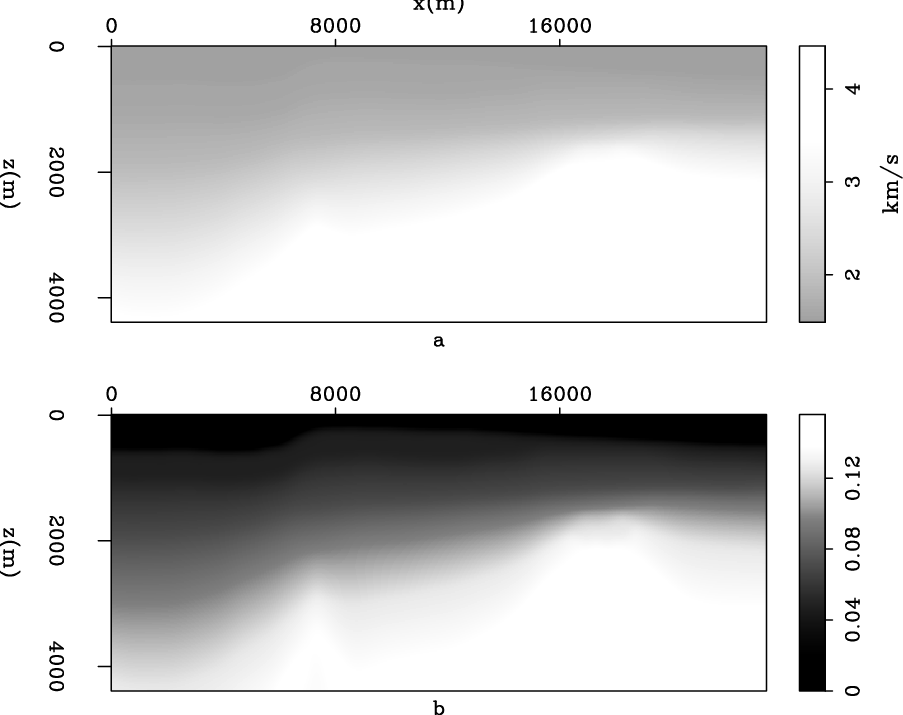
Figure 7. Inversion results using velocity parametrization, expressed in vertical velocity and $\epsilon$ . a): velocity model; b): $\epsilon$ model.

invmodsebw
Figure 8. Inversion results using logarithmic slowness parametrization, expressed in vertical velocity and $\epsilon$ . a): velocity model; b): $\epsilon$ model.

For velocity parametrization, the gradient for vertical velocity has more terms than the gradient for horizontal velocity. This leads to more updates for vertical velocity than for horizontal velocity and tends to result in the epsilon update having a sign opposite to that of the vertical velocity update. Since this is not always geologically true, such inversion model parametrization is not ideal, at least for gradient-based inversion methods. Inversion using logarithmic slowness parametrization results in reasonable data matching; however, relatively smooth $\epsilon$ updates in the inversion result do suggest data misfit from ambiguity between $\epsilon$ changes and vertical velocity changes. This ambiguity can potentially be mitigated by proper model styling.

resdbw
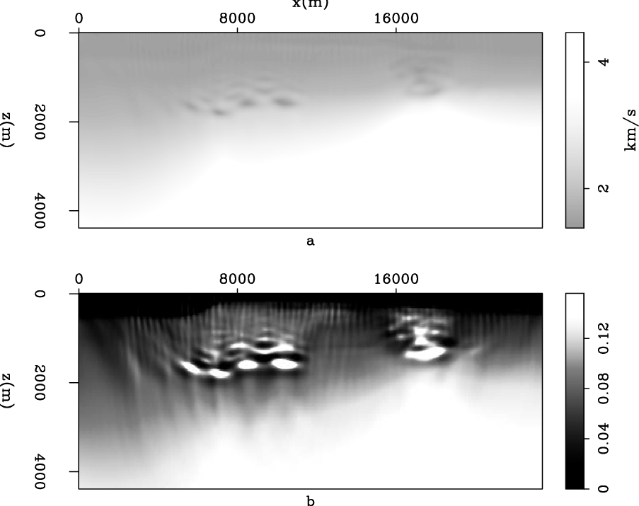
Figure 9. Data residual as a function of iteration number during inversion using different inversion model parametrizations. Continuous: velocity parametrization; dashed: logarithmic slowness parametrization.

For comparison, isotropic inversion is also performed on this model. Two types of starting velocity are used: one is the same vertical velocity model as the starting model in joint inversion, and the other is the horizontal velocity model calculated from the vertical velocity and $\epsilon$ of the starting model used in joint inversion. The inversion results and data misfit are shown in Figures 11 and 12. It is obvious that inversion results are more geologically reasonable starting from the smooth vertical velocity model. This is also supported by data misfit. Comparing results with the true vertical velocity model and the true horizontal velocity model (Figure 10), it is interesting to see that in the better inversion result, the shallow parts mostly agree with the true vertical velocity model, and the deeper parts mostly agree with the true horizontal velocity model.

isomodbw
Figure 10. True velocity model. a): vertical velocity; b): horizontal velocity.

isoinvbw
Figure 11. Velocity model from isotropic inversion starting from, a): smooth vertical velocity; b): smooth horizontal velocity.

isoresdbw
Figure 12. Data residual as a function of iteration during isotropic inversion using different starting models. Continuous: starting from smooth vertical velocity; dashed: starting from smooth horizontal velocity.

Early-arrival waveform inversion for near-surface velocity and anisotropic parameters: inversion of synthetic data