|
|
|
|
Joint imaging with streamer and ocean bottom data |
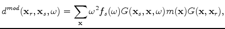
We pose the imaging problem as an inversion problem by linearizing the wave-equation with respect to our model (
 ). Assuming that the earth behaves as a constant-density acoustic isotropic medium, we linearize the wave equation and apply the
first-order Born approximation to get the following forward modeling equation:
). Assuming that the earth behaves as a constant-density acoustic isotropic medium, we linearize the wave equation and apply the
first-order Born approximation to get the following forward modeling equation:
 represents the forward modeled data,
  is the temporal frequency,
represents the reflectivity at image point
is the temporal frequency,
represents the reflectivity at image point
 ,
,
 is the source waveform, and
 is the Green's function of the two-way acoustic constant-density wave equation. Note that
  is actually
dependent. It is important to point out that the adjoint of the forward modeling operator is the migration operator:
is actually
dependent. It is important to point out that the adjoint of the forward modeling operator is the migration operator:
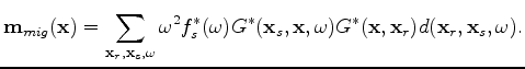 |
(2) |
) is better than the migration image in the sense that its forward-modeled data fits the recorded data.
Next, we discuss how to apply linearized inversion to jointly image with streamer and OBN data.
|
|
|
|
Joint imaging with streamer and ocean bottom data |