Wave-equation migration velocity analysis for anisotropic models on 2-D ExxonMobil field data

Introduction

Compared with isotropic models, anisotropic models are recognized as more realistic representations of the subsurface in complex geological environment. These models are better defined and verified in developing and production areas. However, anisotropic parameters cannot be fully constrained by surface seismic data. Therefore, anisotropic models are better defined in well-developed and production areas, where various well log, check shots and VSP data are available. The ExxonMobil dataset used in this study is from a producing area in an offshore sedimentary basin close to a huge salt body. Figure 1 illustrates the available datasets in this area. While vertical check shots and sonic logs best constrain the vertical velocity model, offset check shot (OCS) data, thanks to its long offset give information on both vertical and horizontal velocity . The current anisotropic model is built using an interactive visualization method (Bear et al., 2005) that integrates surface seismic, sonic logs, vertical check shots, and offset check shots.

alldata
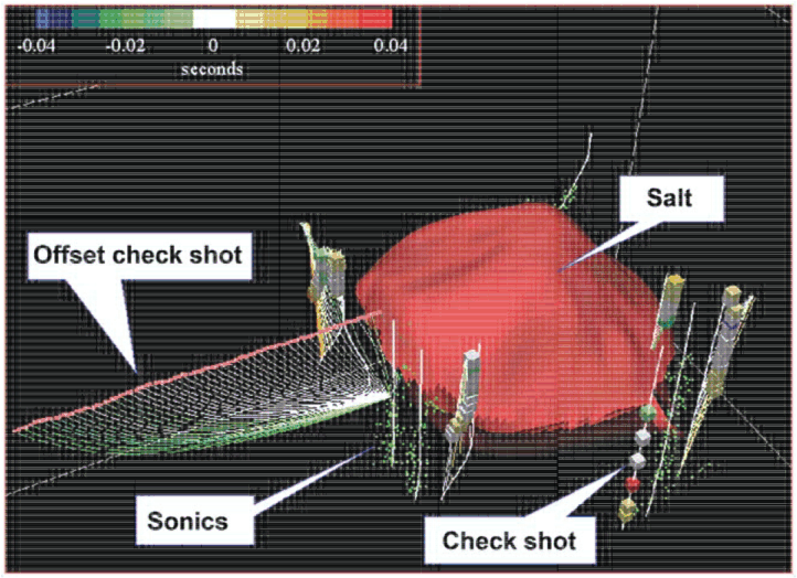
Figure 1. Available datasets for anisotropic model building. From Bear et al. (2005). The current anisotropic model is built using an interactive visualization method that integrates surface seismic, sonic logs, vertical check shots, and offset check shots. The green ray paths show a slower estimation of the velocity and/or a smaller estimation of 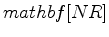$\eta$ .

interact
Figure 2. Visualization of interactive modeling for anisotropy. Top row: Initial isotropic model compared with sonic log and OCS traveltime. APSDM gather is already fairly flat in the small angles. Bottom row: Improved anisotropic model compared with sonic log and OCS traveltime. APSDM gathers are further flattened for large angles. From Bear et al. (2005).

From the results shown in Figure 2, we can see that the anisotropic prestack depth migration (APSDM) gathers are almost flat, inverted velocities have a reasonable match with the sonic logs, and the modeled traveltime agrees with the offset check-shot measurements. However, this interactive visualization method requires human inputs and corrections, which can be cumbersome when large-scale 3-D field data is under examination. Moreover, the most informative data - offset checkshot data - are only acquired sparsely in the 3-D domain, primarily around the salt body. Hence interpolation / extrapolation from these OCS locations is still needed to build a 3-D model elsewhere. This process may lead to inaccurate anisotropic models. Finally, according to the color code in Figure 1, although most of the traveltimes are fitted very well for near- to mid-offset check shots (indicated by rays in white), the travel times modeled between long-offset shots and the downhole receivers are still underestimated compared with the measured travel times (indicated by rays in green). Therefore, a fully automated anisotropic model building method utilizing all types of data would be highly valuable to improve the current model.

To test our method of anisotropic WEMVA (Li and Biondi, 2011), we take a 2-D slice through the sediment basin from this 3-D field dataset where the salt body is far away. The inversion is initialized by the current best model. After 8 iterations, we obtain updated velocity and $\eta$ model that better define the faults in this section and have better continuities in some reflectors.

Wave-equation migration velocity analysis for anisotropic models on 2-D ExxonMobil field data