|
|
|
|
Image gather reconstruction using StOMP |
The most difficult challenge in solving a compressive sensing problem is often finding an effective
 (preferably
  ) solver. These solvers generally have difficulty converging and are
notoriously slow. The large size of any cross-correlation volume (10e7 to 10e8 elements) or,
with a compressed basis still 10e5-10e6, make most
solver approaches impractical.
Donoho et al. (2006) noted this problem with many
approaches and suggested an alternative,
Stagewise Orthogonal Matched Pursuit (StOMP).
) solver. These solvers generally have difficulty converging and are
notoriously slow. The large size of any cross-correlation volume (10e7 to 10e8 elements) or,
with a compressed basis still 10e5-10e6, make most
solver approaches impractical.
Donoho et al. (2006) noted this problem with many
approaches and suggested an alternative,
Stagewise Orthogonal Matched Pursuit (StOMP).
StOMP attempts to leverage the power of  solver with the
properties of approaches
such as basic pursuit (Chen et al., 1998). The basic idea is to iteratively select
the most important model elements by mapping
into the model space and selecting model locations with the largest amplitudes.
An
inversion problem is setup allowing only the locations selected in
the previous step to be non-zero. The problem is mapped back into data space,
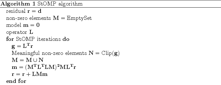
the residual is recalculated, and the process is repeated. Algorithm 1 describes
the approach in more detail.
solver with the
properties of approaches
such as basic pursuit (Chen et al., 1998). The basic idea is to iteratively select
the most important model elements by mapping
into the model space and selecting model locations with the largest amplitudes.
An
inversion problem is setup allowing only the locations selected in
the previous step to be non-zero. The problem is mapped back into data space,
the residual is recalculated, and the process is repeated. Algorithm 1 describes
the approach in more detail.
As a first attempt to use this method, I randomly subsampled a 4-D cr-correlation space (
 )
by a factor of 25 to form
)
by a factor of 25 to form  . I used the multi-dimensional wavelet compression operator
  described
in Clapp (2011), choosing 4 levels in
described
in Clapp (2011), choosing 4 levels in  , 3 levels in
  , 2 levels in
  and
and  as
as  .
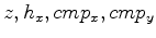
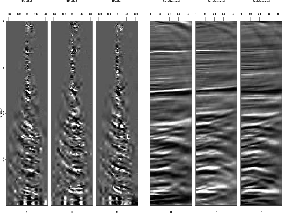
Figure 4 shows two Common Reflection Point (CRP) gathers in the subsurface offset and angle domain. Figure 5
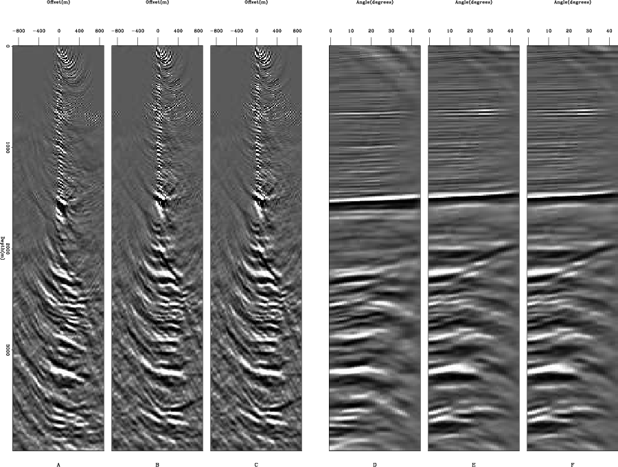
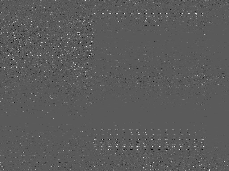
shows a portion of the wavelet domain representation of the cross-correlation gathers, note how few samples
are non-zero.
.
Figure 4 shows two Common Reflection Point (CRP) gathers in the subsurface offset and angle domain. Figure 5
shows a portion of the wavelet domain representation of the cross-correlation gathers, note how few samples
are non-zero.
|
|---|
|
data-init
Figure 4. A, B,C and show two subsurface offset gathers from a 4-D volume. D, E, and F show the same to CRP gathers in the angle domain. |
|
|
|
wavelet
Figure 5. The wavelet domain representation of the subsurface offset domain 4-D volume partially shown in A and B of Figure 4. |
|
|---|---|
|
|
The ``art'' of StOMP is choosing the number of iterations and the clipping scheme to use to select important basis elements. In this example, I took a rather crude approach. I did StOMP iterations increasing the number selected non-zero elements to approximately match the level of sparsity observed in the wavelet domain representation. Figure 6 shows the same two subsurface offset gathers and their corresponding angle gathers. I used a large value clipping scheme that guaranteed 4% non-zero basis elements after 10 iterations Clapp (2011) showed that subsurface offset gathers could be compressed by a factor of 100 and still retain most relevant information. Note that though there is visible noise in the subsurface offset gathers the angle domain representation is quite similar. Figure 7 shows the resulting wavelet domain which appears to be significantly dissimilar to Figure 5. From C and D of Figure 6 however it appears that most of this difference doesn't map into coherent events in the angle domain.
|
|---|
|
data-0
Figure 6. A, B, and C show the recovered subsurface offset gathers using compressive sensing as shown in plot A, B, and C of Figure 4. D, E, and F show the corresponding angle gathers. Note how even though A, B, and C are significantly different than A, B, and C of Figure 4, D, E, and F contain virtually the same information. |
|
|
|
wavelet-try1
Figure 7. The wavelet domain signal after 10 iterations of StOMP. Note the dissimilarity with the correct wavelet domain show in Figure 5. |
|
|---|---|
|
|
|
|
|
|
Image gather reconstruction using StOMP |