Preconditioning a non-linear problem and its application to bidirectional deconvolution

Preconditioning offers smart directions

We start from fitting goals

$$\begin{gathered}{\mathbf{0}} \approx {\mathbf{Fm}} - {\mathbf... ... \\ {\mathbf{0}} \approx {\mathbf{Am}} \hfill \\ \end{gathered}$$ (1)

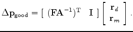
and change variables from ${\mathbf{m}}$ to ${\mathbf{p}}$ using ${\mathbf{m}} = {\mathbf{A}}^{ - 1} {\mathbf{p}}$ :

$$\begin{gathered}{\mathbf{0}} \approx {\mathbf{r}}_d = {\mathb... ...r}}_m = {\mathbf{Am}} = {\mathbf{Ip}} \hfill. \\ \end{gathered}$$ (2)

Without preconditioning, we have the search direction

$$\Delta {\mathbf{m}}_{{\text{bad}}} = [\begin{array}{*{20}c} {{\ma... ...}{*{20}c} {{\mathbf{r}}_d } \\ {{\mathbf{r}}_m } \\ \par \end{array} } \right],$$ (3)

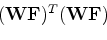
and with preconditioning, we have the search direction

$$\Delta {\mathbf{p}}_{{\text{good}}} = [\begin{array}{*{20}c} {({\... ...}{*{20}c} {{\mathbf{r}}_d } \\ {{\mathbf{r}}_m } \\ \par \end{array} } \right].$$ (4)

The essential feature of preconditioning is not that we perform the iterative optimization in terms of the variable ${\mathbf{p}}$ , but that we use a search direction that is a gradient with respect to ${\mathbf{p}}^{\rm T}$ , not ${\mathbf{m}}^{\rm T}$ . Using ${\mathbf{Am}} = {\mathbf{p}}$ we have ${\mathbf{A}}\Delta {\mathbf{m}} = \Delta {\mathbf{p}}$ . This enables us to define a good search direction in model space:

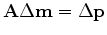$$\Delta {\mathbf{m}}_{{\text{good}}} = {\mathbf{A}}^{ - 1} \Delta ... ...m T} {\mathbf{F}}^{\rm T} {\mathbf{r}}_d + {\mathbf{A}}^{ - 1} {\mathbf{r}}_m .$$ (5)

We define the gradient by ${\mathbf{g}} = {\mathbf{F}}^{\rm T} {\mathbf{r}}_d$ and notice that ${\mathbf{r}}_m = {\mathbf{p}}$ .

$$\Delta {\mathbf{m}}_{{\text{good}}} = {\mathbf{A}}^{ - 1} ({\mathbf{A}}^{ - 1} )^{\rm T} {\mathbf{g}} + {\mathbf{m}}.$$ (6)

The search direction (6) shows a positive-definite operator scaling the gradient. All components of any gradient vector are independent of each other and independently point to a direction for descent. Obviously, each can be scaled by any positive number. Now we have shown that we can also scale a gradient vector by a positive definite matrix and still expect the conjugate-direction algorithm to descend, as always, to the ``exact'' answer in a finite number of steps. This is because modifying the search direction with ${\mathbf{A}}^{ - 1} ({\mathbf{A}}^{ - 1} )^{\rm T}$ is equivalent to solving a conjugate-gradient problem in ${\mathbf{p}}$ .

Preconditioning a non-linear problem and its application to bidirectional deconvolution