Preconditioning a non-linear problem and its application to bidirectional deconvolution

Introduction

Least-squares data fitting leads to multivariate linear equations and consequently more theories and techniques than any one person can master in a lifetime. In that field, we are always on well-traveled paths. Problems with non-linear physics are another story: ``My program worked great until I increased the model size a little bit.''

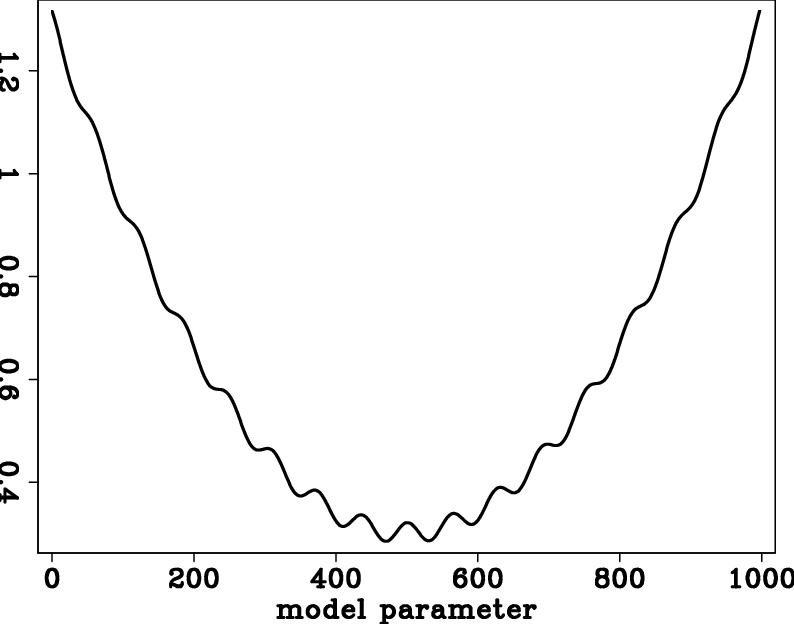
Nonlinear optimization problems have many unexpected traps--local minima, as shown in Figure 1. Problems with nonlinear physics require a deeper understanding of the setting than do linear ones. Luckily, there exist helpful techniques that are universally applicable. The first key is to realize that linear equations can be solved with any starting guess, whereas with nonlinear relationships, a sensible starting solution is essential.

Preconditioning is a well established technique used in linear regressions with prior information to hasten convergence. Preconditioning usually begins with regularization and then steers the iterative descent along the path set out by a prior model. However, it does not determine the final result.

The word ``gradient'' sounds like something fixed in the geometry of the application. Nothing could be further from the truth. Every application offers us a choice of coordinate systems and ways to parameterize the model, and changing the model representation changes the gradient. For example, we could be seeking the earth density as a function of location. We could establish the problem as just that, density as a function of location. On the other hand, we could establish the problem as finding the spatial derivative of the density. The two formulations really seek the same thing, but operators, unknowns, and gradients differ.

Each component of a gradient is independent of the other components and may be scaled arbitrarily as long as its polarity is unchanged. That means that any gradient can be multiplied by any diagonal matrix containing all positive numbers. Additionally, we show in the theory section below that a gradient may be multiplied by any positive definite matrix. That matrix happens to be the model covariance ${\bf B}^T{\bf B}$ , which in local terminology is the inverse of the model styling goal times its adjoint. We may choose any positive definite matrix to modify the gradient. We may even change that matrix from one iteration to the next. What is important is that the matrix is positive definite. At early stages of descent, it is helpful to make the gradient large where confidence is high, and small where it is not. With linear regressions this has no effect on the solution. With nonlinear physics, it steers the solution away from unwelcome local minima.

In image estimation there generally are locations in physical space and in Fourier space in which we have little interest, where we have little expectation that our data contains useful information or that the model will be findable. We need (in nonlinear cases) to be certain such regions do not disturb our descent, especially in early iterations. Therefore, we should view our gradient both in the model space and in the data space, then choose an appropriate diagonal weighting and filter. Given a filter ${\bf F}$ and weight ${\bf W}$ , we apply either ${\bf F}{\bf W}$ or ${\bf W}{\bf F}$ to the gradient. We then apply the matrix transpose, yielding either $({\bf F}{\bf W})^T({\bf F}{\bf W})$ or $({\bf W}{\bf F})^T({\bf W}{\bf F})$ . This procedure destroys no information in the data, but merely selects what aspects of the data are used first. As the final solution is approached, the gradient diminishes; and the down-weighted regions eventually emerge in the gradient, because they are the only things left. Closer to the ultimate solution, it is far less dangerous to have down-weighted regions affecting the solution.

wigglypar Figure 1. Multiple local minima in the penalty function.

Preconditioning a non-linear problem and its application to bidirectional deconvolution