Krylov space solver in Fortran 2009: Beta version

Example

Converting RMS velocities to interval velocities is one of the most basic problems in reflection seismology. The Dix equation is one of the most common approaches but often leads to unrealistic velocities when dealing with the noise in the RMS velocity measurement. Clapp et al. (1998) points out that there is a linear relationship between $\bf v_{\rm rms}^2$ and $\bf v_{\rm int}^2$ using either a modified version of causal integration or using causal integration $\bf C$ directly and first scaling $\bf v_{\rm rms}^2$ by sample number. With this linear relation we can now add a model styling goal, such as smooth $\bf v_{\rm int}^2$ , given us the fitting goals

$$\bf d \approx \bf C \bf m$$ (10)

$$\bf0 \approx \epsilon \bf D \bf m,$$

where $\bf D$ is the derivative operator, $\bf d$ is the scaled $\bf v_{\rm rms}^2$ , and the model is $\bf v_{\rm int}^2$ . We need a weighting term which gives higher importance to good RMS picks, and equal weights all of the RMS velocities (undoing the effect of the sample number scaling), resulting in

$$\bf0 \approx \bf W( \bf d - \bf C \bf m)$$ (11)

$$\bf0 \approx \epsilon \bf D \bf m.$$

We can precondition the model by noting that causal integration is the inverse of the derivative except at the first sample. We know that first interval velocity value is the same as the first RMS velocity, resulting in the final setting of fitting equations,

$$\bf0 \approx \bf W( \bf d - \bf C \bf\bf M \bf p)$$ (12)

$$\bf0 \approx \epsilon \bf p,$$

where $\bf p$ is the preconditioned variable and $\bf M$ is a masking operator that doesn't allow the first value to change. The advantage of selecting this problem is that its solution is a rather thorough test of all the necessary features of the solver. It involves a starting model, a weighting operator, and a masking operator. It requires both chaining operators and making column operator objects. All of the hard stuff is done away from the user in the solver, the user only needs to construct the required operators and initialize and run the solver.

For this example the conversion is all handled in a module. The module begins by using all of the modules that declare the operators and solvers, and the declaration of variables.

module vrms_2_int_mod !Transform from RMS to interval velocity
  use causint_mod  !Causal integration
  use weight_mod   !Weighting operator
  use mask_mod     !Masking operator
  use cg_step_mod  !Conjugate gradient
  use obj_solver_mod !Solver module
contains
  subroutine vrms2int( niter, eps, weight, vrms, vint)
    integer,            intent( in)     :: niter     ! iterations
    real,               intent( in)     :: eps       ! scaling parameter
    type(real_1d)                       :: vrms      ! rms velocity
    type(real_1d),target                       :: vint! interval velocity
    real, dimension(:), pointer         :: weight    ! data weighting
    integer                             :: st,it,nt
    logical, dimension( size( vint%vals))    :: mask
    logical, dimension(:), pointer      :: msk
    real,    dimension( size( vrms%vals))    :: wt
    real, dimension(:), pointer         :: wght
    type(prec_solver)  :: p_s   !Preconditioned solver

    type(causint_op),target :: ca_op,ca2_op   !Causal integration
    type(mask_op),target    :: m_op           !Masking operator

    type(weight_op),target :: wt_op   !Weighting operator
    type(cgstep),target :: cg   !Conjugate gradient operator
    type(real_1d),target :: dat  !Data

Next we need to scale the data, create the weighting vector, and masking vector.

vrms2int.f90        vrms2int.unrat      vrms_2_int_mod.mod  
    nt = size( vrms%vals)
   
    call create_vec1(dat,vrms%vals)
         do it= 1, nt
           dat%vals( it) = vrms%vals( it) * vrms%vals( it) * it
           wt( it) = weight( it)*(1./it)           ! decrease weight with time
         end do
    
    mask = .false.;   mask( 1) = .true.            ! constrain first point
    vint%vals = 0.     ;   vint%vals(1)= dat%vals( 1)
    
    allocate(msk(size(mask)))
    msk=.not.mask

    allocate(wght(size(wt)))
    wght=wt

Finally we need to initialize the operators, setup the solver, and solve for the interval velocity squared.

    call create_weight_op(wt_op,vrms,wght) !Create weighting op
    call create_causint_op(ca_op,vint,"a1") !Causal op
    call create_causint_op(ca2_op,vint,"a2")!Preconditioning
    call create_mask_op(m_op,vint,msk)  !Masking operator

    p_s%lop=>ca_op;   !Mapping operator
    p_s%st=>cg;       !Step function
    p_s%pop=>ca2_op   !Preconditioning operator
    p_s%dat=>dat;     !Data
    p_s%mod=>vint     !model
    p_s%jop=>m_op;    !Masking operator
    p_s%wop=>wt_op    !Weighting operator
    p_s%eps=eps;      !Scaling factor
    p_s%p0=>vint      !Initial preconditioned variable
    call p_s%solve(niter)  !Solve for interval v^2

    call ca_op%op(.false.,.false.,vint,dat)  !Estimated RMS^2

    do it= 1, nt
       vrms%vals( it) = sqrt( dat%vals( it)/it)  !RMS velocity
    end do
    vint%vals = sqrt( vint%vals) !Interval velocity
    deallocate(wght); deallocate(msk)
 end subroutine
 end module

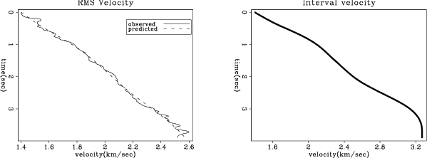
Figure 2 shows the result of running the inversion. The left panel shows the original RMS velocity and the mapped RMS velocity. The right panel shows the estimated interval velocity.

stiff
Figure 2. The left panel shows the original RMS velocity and the mapped RMS velocity. The right panel shows the estimated interval velocity.

Krylov space solver in Fortran 2009: Beta version