|
|
|
|
Two-parameters residual-moveout analysis for wave-equation migration velocity analysis |
What I call the Taylor RMO function adds the next higher-order even term to equation 1 as follows
The second two-parameter RMO function that I introduce adds a sine function to equation 1 as follows
|
|---|
|
Cig
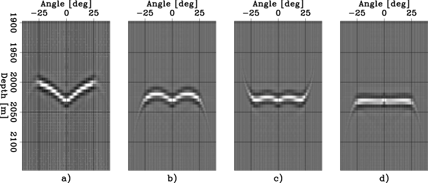
Figure 1. CIGs after constant velocity migration and: a) no correction, b) correction with a one-parameter RMO (equation 1), c) correction with the ``Taylor'' RMO (equation 2), and d) correction with the ``Orthogonal'' RMO (equation 3). |
|
|
Figure 1a shows the first CIG that I use
for my study.
It was obtained by migrating a synthetic data set
that was modeled assuming a strong negative velocity anomaly
above a flat reflector
and migrated assuming a constant velocity
(Biondi, 2011).
This CIG is located under the center of the anomaly.
Its moveout is not well described by the conventional RMO
function expressed in equation 1 because the image
at near angles is more affected by the anomaly
than the image at far angles.
Figure 1b shows the result of
correcting this CIG using equation 1
with
![]() that is the
that is the ![]() value corresponding
to the maximum of the stack power picked from a stack-power spectrum.
This corrected CIG is far from being flat.
value corresponding
to the maximum of the stack power picked from a stack-power spectrum.
This corrected CIG is far from being flat.
|
|---|
|
Smooth
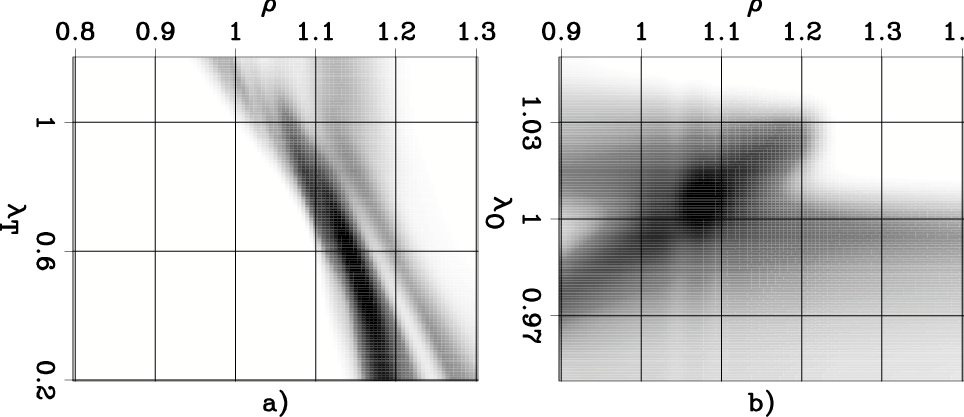
Figure 2. Two-parameter stack-power spectra resulting from RMO analysis of the migrated CIG shown in Figure 1a obtained applying: a) the ``Taylor'' RMO function (equation 2), and b) the ``Orthogonal'' RMO function (equation 3). |
|
|
The maxima of both of these two-parameter spectra are not along
the ![]() line, indicating that the two-parameter RMO improves
the flatness with respect to the one-parameter RMO.
Indeed, when the values corresponding to the maxima of the
power spectra shown
in Figure 2
are used to correct the original CIG I obtain
flatter gathers than when using a one-parameter RMO.
Figure 1c shows the result of
correcting the CIG shown Figure 1a
using equation 2
with
line, indicating that the two-parameter RMO improves
the flatness with respect to the one-parameter RMO.
Indeed, when the values corresponding to the maxima of the
power spectra shown
in Figure 2
are used to correct the original CIG I obtain
flatter gathers than when using a one-parameter RMO.
Figure 1c shows the result of
correcting the CIG shown Figure 1a
using equation 2
with ![]() and
and
![]() .
Figure 1c shows the result of
correcting the CIG shown Figure 1a
using equation 3
with
.
Figure 1c shows the result of
correcting the CIG shown Figure 1a
using equation 3
with
![]() and
and
![]() .
The CIG corrected using the ``Orthogonal'' RMO is almost perfectly
flat within the
.
The CIG corrected using the ``Orthogonal'' RMO is almost perfectly
flat within the
![]() range.
range.
Notice that the shape of the spectra around their respective maxima is substantially different between the two plots. The function corresponding to the ``Orthogonal'' RMO is more isotropic around the maximum than the one corresponding to the ``Taylor'' RMO. This behavior is expected because the two terms of the ``Orthogonal'' RMO function are close to be orthogonal with respect to each other. Theoretically, this more isotropic shape could lead to better gradients. However, we can also notice diagonal artifacts in Figure 2b. As we discuss below, the effects of these artifacts tend to outweigh any advantage provided by the more isotropic shape of the spectrum.
|
|---|
|
Cig-aniso
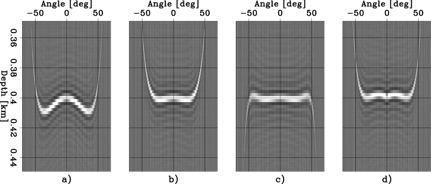
Figure 3. CIGs after isotropic velocity migration and: a) no correction, b) correction with a one-parameter RMO (equation 1), c) correction with the ``Taylor'' RMO (equation 2), and d) correction with the ``Orthogonal'' RMO shows the second CIG that I use (equation 3). |
|
|
Figure 3a shows the second CIG that I use
for my analysis.
It was obtained by migrating a synthetic data set
that was modeled assuming a strongly anisotropic VTI
medium (
![]() and
and
![]() )
above a flat reflector,
and migrated assuming an isotropic velocity
(Biondi, 2005).
Because the anisotropy in the medium is not taken into account
by the isotropic migration,
the CIG moveout is not well described by the conventional
one-parameter RMO
function expressed in equation 1.
Figure 1b shows the result of
correcting this CIG using equation 1
with
)
above a flat reflector,
and migrated assuming an isotropic velocity
(Biondi, 2005).
Because the anisotropy in the medium is not taken into account
by the isotropic migration,
the CIG moveout is not well described by the conventional
one-parameter RMO
function expressed in equation 1.
Figure 1b shows the result of
correcting this CIG using equation 1
with
![]() that is the
that is the ![]() value corresponding
to the maximum of the stack power picked from a stack-power spectrum.
This corrected CIG is far from being flat.
value corresponding
to the maximum of the stack power picked from a stack-power spectrum.
This corrected CIG is far from being flat.
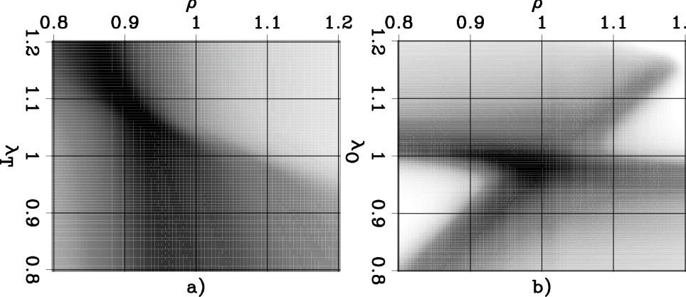
Figure 4 shows
stack-power spectra as a function
of two parameters.
The panel on the left (Figure 4a)
was computed using
the ``Taylor'' RMO function described by equation 2,
whereas
the panel on the right (Figure 4b)
was computed using
the ``Orthogonal'' RMO function described by equation 3.
In both cases the stack power was computed over the
range of
![]() .
Consequently,
I set
.
Consequently,
I set
![]() to compute the normalized angle
to compute the normalized angle
![]() in equation 3.
The power spectra were averaged over a thick (200 m)
depth interval and slightly smoothed along the RMO
parameters
in equation 3.
The power spectra were averaged over a thick (200 m)
depth interval and slightly smoothed along the RMO
parameters ![]() and
and ![]() .
.
|
|---|
|
Smooth-aniso
Figure 4. Two-parameter stack-power spectra resulting from RMO analysis of the migrated CIG shown in Figure 3a obtained applying: a) the ``Taylor'' RMO function (equation 2), and b) the ``Orthogonal'' RMO function (equation 3). |
|
|
As for the spectra computed from the first CIG (Figure 2), the function corresponding to the ``Orthogonal'' RMO is more isotropic around the maximum than the one corresponding to the ``Taylor'' RMO. This difference in shape is less pronounced for this example than for the previous one.
Because the maxima of both of these two-parameter spectra are not along
the ![]() line, we have indication that the two-parameter RMO improves
the flatness with respect to the one-parameter RMO.
Indeed, when the values corresponding to the maxima of the
power spectra shown
in Figure 4
are used to correct the original CIG I obtain
flatter gathers than when using a one-parameter RMO.
Figure 3c shows the result of
correcting the CIG shown Figure 3a
using equation 2
with
line, we have indication that the two-parameter RMO improves
the flatness with respect to the one-parameter RMO.
Indeed, when the values corresponding to the maxima of the
power spectra shown
in Figure 4
are used to correct the original CIG I obtain
flatter gathers than when using a one-parameter RMO.
Figure 3c shows the result of
correcting the CIG shown Figure 3a
using equation 2
with
![]() and
and
![]() .
Figure 3c shows the result of
correcting the CIG shown Figure 3a
using equation 3
with
.
Figure 3c shows the result of
correcting the CIG shown Figure 3a
using equation 3
with ![]() and
and
![]() .
In particular,
the CIG corrected using the ``Taylor'' RMO is significantly
flatter,
within the
.
In particular,
the CIG corrected using the ``Taylor'' RMO is significantly
flatter,
within the
![]() range,
than the one corrected using a one-parameter RMO.
range,
than the one corrected using a one-parameter RMO.
|
|
|
|
Two-parameters residual-moveout analysis for wave-equation migration velocity analysis |