Elastic wavefield directionality vectors

Polarization coefficient and displacement decomposition in the wavenumber and space domain

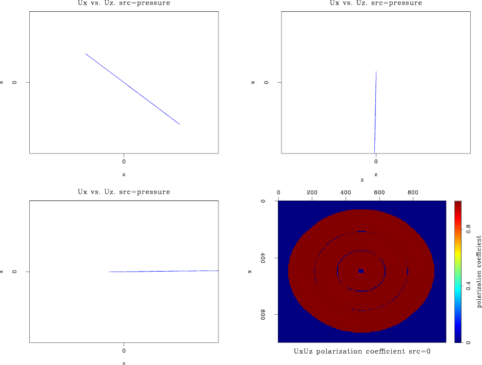
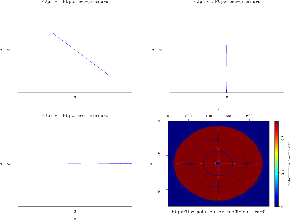
The bottom right of Figure 5 is the polarization coefficient (equation 25) of the pressure-source wavefield (Figure 3), calculated at time $T = 200$   ms . The time window size in which the polarization coefficient was calculated was $90$   ms , with its center at $T = 200$   ms . The polarization coefficient is clipped below $r=0.8$ , which means that the field shows only model locations with very high polarization (clipped values are blue). As we may expect, this being a solitary pressure wave in a homogeneous medium, the field is indeed very linearly polarized.
The other panels in Figure 5 show crossplots (hodograms) of the vertical and horizontal displacement, in various locations in the wavefield within the time window centered at $T = 200$   ms . For a linearly polarized wave, we expect this crossplot to appear as a thin line (the effect of linear dependence between displacement components). Otherwise, we should see an irregular shape in the crossplot. The panel on the bottom left of Figure 5 is the displacement crossplot at the center-left of the wavefield. The upper left panel is the displacement crossplot near the upper left corner of the wavefield, and the upper right panel is displacement at the center-top of the wavefield. Since there is only a single propagating P-wave present in the wavefield, all these locations exhibit linear dependence between the displacement components, indicating a high degree of polarization. The fundamental characteristic of P-waves, that the particle motion is tangent to the wave propagation direction, can be seen from this figure. All the crossplots seem to ``radiate'' away from the source, since there is only one source at the center. This is a demonstration of how polarization of displacements indicates the wavefield's directionality.

0Uxzpol Figure 5. Bottom right: Polarization coefficient for a pressure source clipped below $r=0.8$ , and $U_x$ vs. $U_z$ displacement crossplots at certain locations in the wavefield at $T = 208$   ms . Bottom left: crossplot at $x=500,z=330$ . Top left: crossplot at $x=330,z=330$ . Top right: crossplot at $x=330,z=500$ .

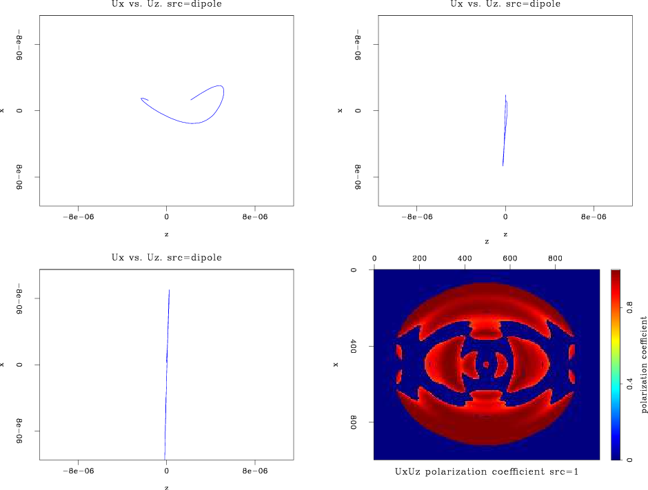
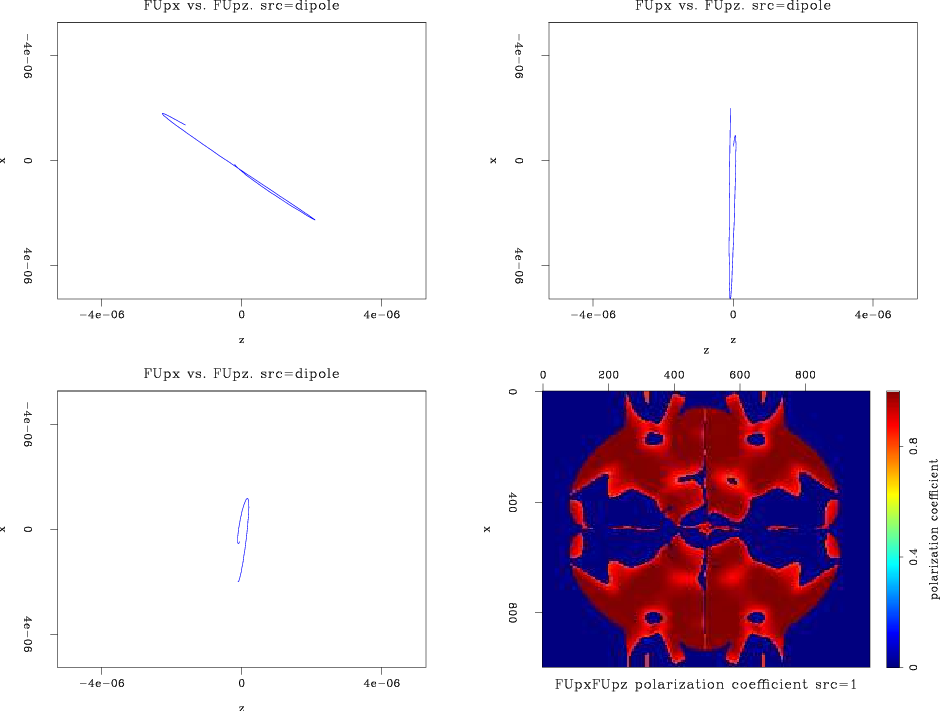
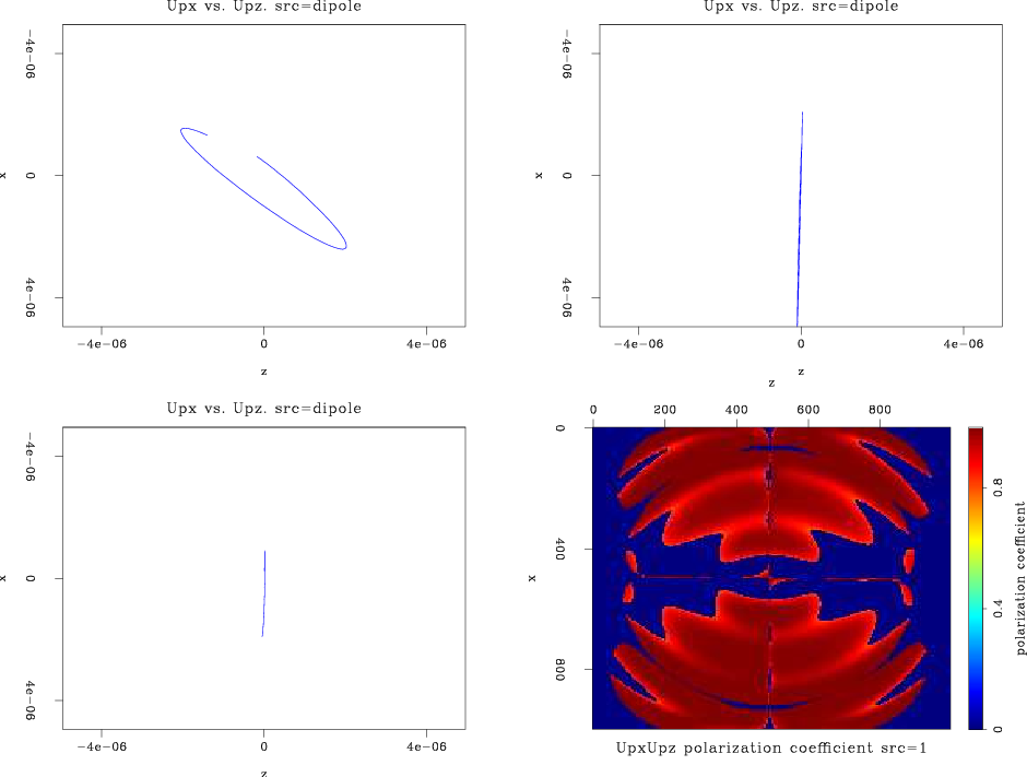
Figure 6 displays the same panels as Figure 5, but in this case the source is a dipole source in the vertical direction, meaning that the displacement in the vertical axis $(U_x)$ at the center of the wavefield is being forced. This results in the P and S waves shown in Figure 4. For this source, the polarization coefficient exhibits large regions of non-polarized waves, as seen by the polarization coefficient map on the bottom right of Figure 6. Examining the surrounding crossplot panels, a different picture of polarization appears: where in Figure 5 the polarization on the left of the model is horizontal, in Figure 6 it is vertical. The reason for this is that when a dipole source is excited, the wavefield contains a mixture of P and S waves, and thus a mixture of P and S displacements, as seen in Figure 4. Therefore, the linear polarization crossplot on the bottom left panel of Figure 6 is a result of shear wave displacements, while the linear polarization crossplot on the top right is a result of pressure wave displacements. The shear wave and its associated vertical particle motion propagates in the horizontal direction, while the pressure wave and its associated vertical particle motion propagates vertically. Consequently, the panel on the top left of Figure 6, which displays the crossplot at the upper left corner of the wavefield, is a mixture of shear and pressure displacements, and therefore exhibits particle motion which is not linearly polarized. This figure shows the need for a displacement decomposition method.

1Uxzpol Figure 6. Bottom right: Polarization coefficient for a vertical dipole source clipped below $r=0.8$ , and $U_x$ vs. $U_z$ displacement crossplots at certain locations in the wavefield at $T = 208$   ms . Bottom left: crossplot at $x=500,z=330$ . Top left: crossplot at $x=330,z=330$ . Top right: crossplot at $x=330,z=500$ .

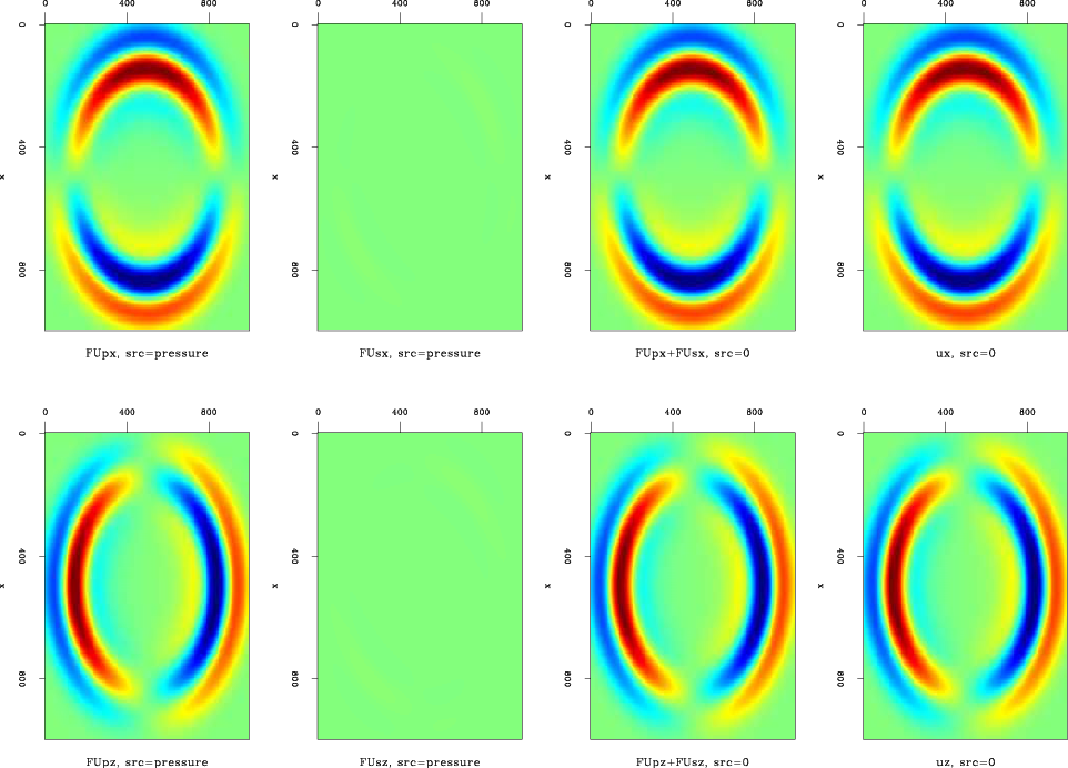
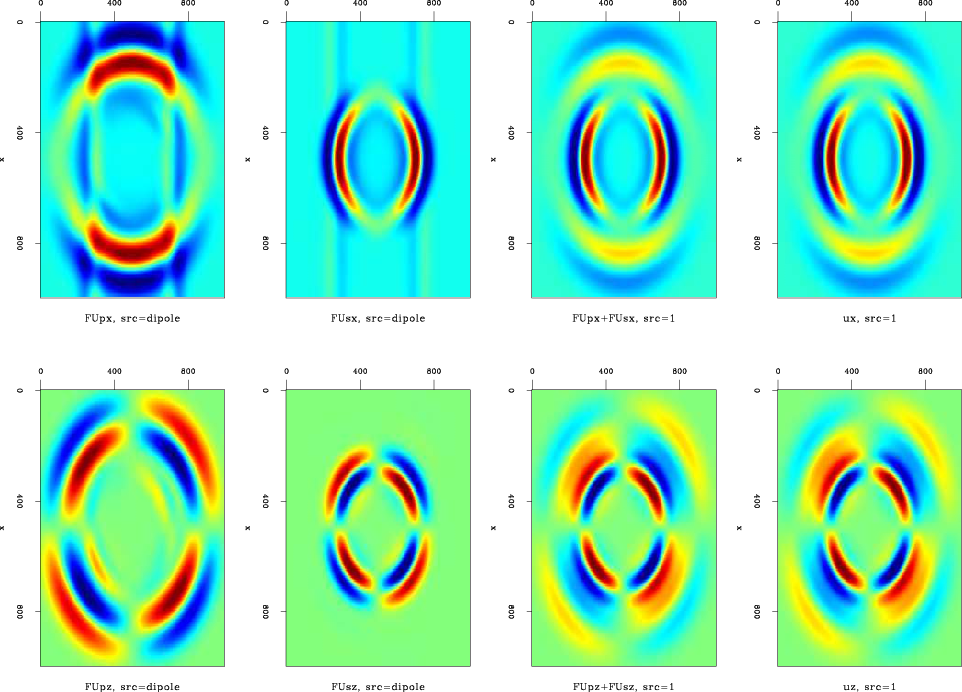
Figure 7 is an example of the implementation of P and S wave displacement decomposition in the wavenumber domain (equations 12 and 14), when a pressure source is applied. Shear waves are not expected to form in this case since the medium is homogeneous. The top row shows the vertical displacements, and the bottom row shows the horizontal displacements. From left to right, the panels are the pressure wave displacements after decomposition $(U^P)$ , the shear wave displacements after decomposition $(U^S)$ , the sum of the shear and pressure displacements $(U^P + U^S)$ , and the original displacements before decomposition. Figure 9 is the same, but in this case the source is a vertical dipole source. The expectation is that the sum of displacements after decomposition will be equal to the displacements before decomposition, and it is does appear to be so.

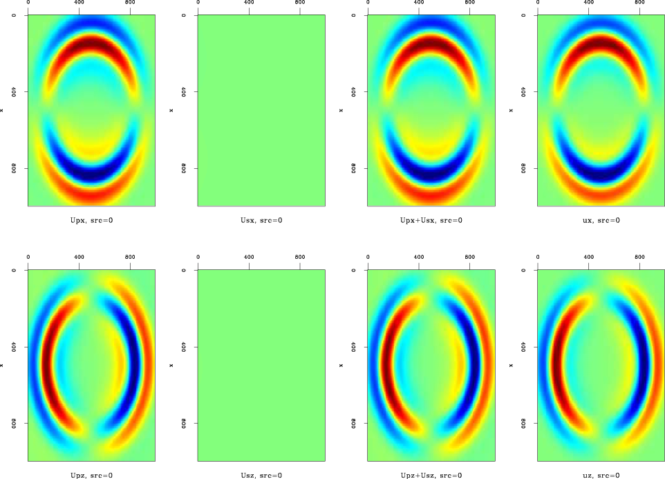
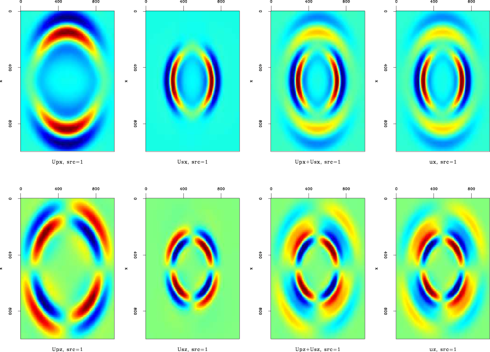
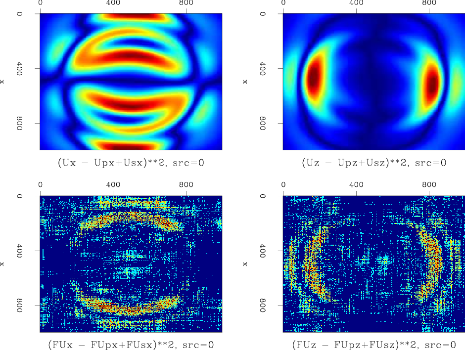
Figure 8 is the implementation of P and S wave displacement decomposition in the space domain (equations 24), when a pressure source is applied. The results are similar to those from the wavenumber domain decomposition, shown in Figure 7. Figure 10 shows the space domain decomposition for a vertical dipole source. In this case, the decomposed displacements are different from those seen by the wavenumber decomposition, shown in Figure 9. Notice the vertical streaks in the top left panels of Figure 9. I interpret these streaks as artifacts of the Fourier transform, since when I use more zero padding before applying the 2D Fourier transform, their magnitude decreases. However, it is interesting that the resulting summations in both cases appear similar, and likewise appear almost identical to the pre-decomposed displacements. This shows that the decomposition method in the wavenumber domain by Zhang and McMechan (2010), and the decomposition in the space domain both work in principle for an isotropic medium.

0Fseparated-combined
Figure 7. Decomposed displacements snapshot at $T = 250 ms$ for a pressure source. Displacement decomposition is in wavenumber domain. X is the vertical direction, Z is horizontal. Top row: displacements in X direction. Bottom row: displacements in Z direction. From left to right: P displacements, S displacements, P+S displacements and original displacements.

0separated-combined
Figure 8. Decomposed displacements snapshot at $T = 250 ms$ for a pressure source. Displacement decomposition is in space domain. X is the vertical direction, Z is horizontal. Top row: displacements in X direction. Bottom row: displacements in Z direction. From left to right: P displacements, S displacements, P+S displacements and original displacements.

1Fseparated-combined
Figure 9. Decomposed displacements snapshot at $T = 250 ms$ for a vertical dipole source. Displacement decomposition is in wavenumber domain. X is the vertical direction, Z is horizontal. Top row: displacements in X direction. Bottom row: displacements in Z direction. From left to right: P displacements, S displacements, P+S displacements and original displacements.

1separated-combined
Figure 10. Decomposed displacements snapshot at $T = 250 ms$ for a vertical dipole source. Displacement decomposition is in space domain. X is the vertical direction, Z is horizontal. Top row: displacements in X direction. Bottom row: displacements in Z direction. From left to right: P displacements, S displacements, P+S displacements and original displacements.

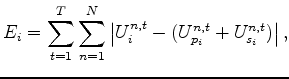
However, a large difference between the wavenumber and space domain methods appears when comparing the errors of the sum of the decomposed displacement fields vs. the pre-decomposed displacement fields. The comparison is done by calculating the absolute value of the difference between the summed-decomposed displacements and the undecomposed displacements for each model point at each propagation time, and then summing all that into a single number:

$$E_i = \sum_{t=1}^T \sum_{n=1}^N \left\vert U^{n,t}_i - (U^{n,t}_{p_i} + U^{n,t}_{s_i}) \right\vert,$$ (30)

where $U^{n,t}_i$ is the displacement in direction $i$ before decomposition, at model point $n$ at propagation time $t$ , $U^{n,t}_{p_i}$ is the decomposed P wave displacement, and $U^{n,t}_{s_i}$ is the decomposed S wave displacement. Figures 11 and 12 show a comparison of the absolute difference field at $T = 200 ms$ for the wavenumber and space domain decompositions. The figures are misleading, since the maximum value of the wavenumber domain difference is $6$ orders of magnitude less than the space domain decomposition difference. The expectation is that the sum of displacements after decomposition will be equal to the displacements before decomposition. It appears that this is the case for decomposition in the wavenumber domain, at least from the relative error point of view.
The following table shows the summations of the absolute displacement fields and the absolute decomposition errors, over the entire propagation time, for a pressure source and a dipole source:

Source	$\left\vert U_x \right\vert$	$E_x \,$   space	Rel. err	$E_x \,$   wavenumber	Rel. err
Pressure	3.54e-10	5.51e-11	0.15	6.06e-17	0.17e-6
Dipole	5.19	0.88	0.17	1.68e-6	0.32e-6
Source	$\left\vert U_z \right\vert$	$E_z \,$   space	Rel. err	$E_z \,$   wavenumer	Rel. err
Pressure	3.54e-10	7.56e-11	0.21	5.95e-17	0.16e-6
Dipole	3.32	0.36	0.10	1.03e-6	0.31e-6

0space-vs-wavenumber-diff Figure 11. Absolute errors of decomposed displacements in comparison to original displacements for a pressure source. $T = 250$   ms . Top: displacement decomposition in space domain. Bottom: displacement decomposition in the wavenumber domain. Wavenumber domain errors are 6 orders of magnitude smaller than space domain.

1space-vs-wavenumber-diff Figure 12. Absolute errors of decomposed displacements in comparison to original displacements for a vertical dipole source. $T = 250$   ms . Top: displacement decomposition in space domain. Bottom: displacement decomposition in the wavenumber domain. Wavenumber domain errors are 6 orders of magnitude smaller than space domain.

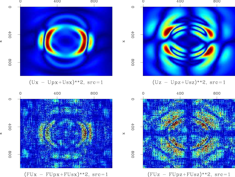
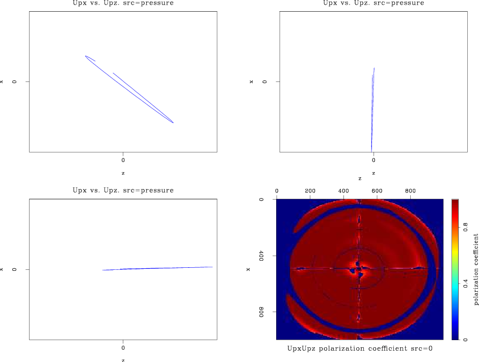
The correctness of the displacement decomposition operators can be verified when comparing Figure 5 to Figures 13 and 14. Since there is only a pressure wave in the wavefield, we expect the decomposition operator to not have an effect on the resulting pressure wave polarization. Looking at these two figures, we can see they are similar, indicating that the decomposition operators do not introduce a significant amount of numerical inaccuracies. However, it is clear that decomposition in the wavenumber domain has introduced less errors into the P wave displacements.

0FUpxzpol Figure 13. Bottom right: Polarization coefficient for a pressure source clipped below $r=0.8$ , and $U^{P}_x$ vs. $U^{P}_z$ displacement crossplots at certain locations in the wavefield at $T = 208$   ms . Decomposition is in the wavenumber domain. Bottom left: crossplot at $x=500,z=330$ . Top left: crossplot at $x=330,z=330$ . Top right: crossplot at $x=330,z=500$ .

0Upxzpol Figure 14. Bottom right: Polarization coefficient for a pressure source clipped below $r=0.8$ , and $U^{P}_x$ vs. $U^{P}_z$ displacement crossplots at certain locations in the wavefield at $T = 208$   ms . Decomposition is in the space domain. Bottom left: crossplot at $x=500,z=330$ . Top left: crossplot at $x=330,z=330$ . Top right: crossplot at $x=330,z=500$ .

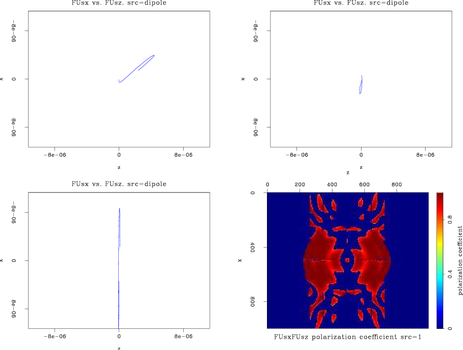
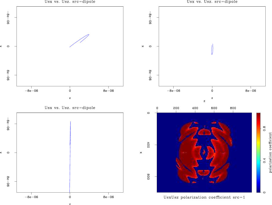
The effect of decomposition on polarization can be seen when comparing Figure 6 to Figures 15 - 18. Notice in particular the top left panel in these figures, indicating the crossplot of vertical and horizontal displacements on the upper left corner of the wavefield. Where in Figure 6 this panel displayed non-linear polarization as a result of a mixture of P and S displacements, in Figures 15 and 16 the polarization appears more linear, similar to the same panel in Figure 5 where only a P wave existed. In Figures 17 and 18, the same panel likewise shows a more linear polarization, but in this case the polarization is flipped by $90$ degrees compared to that in Figure 15. This is exactly what we would expect to see - for a shear wave, the particle motion is perpendicular to the wave's propagation direction. Looking at the bottom left panel of Figures 15 and 16, we can see that the $U^p_x$ displacement amplitude is about $20\%$ of that in the top right panel, since at that location the P displacement should be quite small (refer to Figure 4). Similarly, looking at the top right panel of Figures 17 and 18 we can see that the $U^s_x$ displacement amplitude is significantly lower than in the bottom left panels of these figures. Again - refer to Figure 4 to understand why that should be so.

1FUpxzpol Figure 15. Bottom right: Polarization coefficient for a vertical dipole source clipped below $r=0.8$ , and $U^{P}_x$ vs. $U^{P}_z$ displacement crossplots at certain locations in the wavefield at $T = 208$   ms . Decomposition is in the wavenumber domain. Bottom left: crossplot at $x=500,z=330$ . Top left: crossplot at $x=330,z=330$ . Top right: crossplot at $x=330,z=500$ .

1Upxzpol Figure 16. Bottom right: Polarization coefficient for a vertical dipole source clipped below $r=0.8$ , and $U^{P}_x$ vs. $U^{P}_z$ displacement crossplots at certain locations in the wavefield at $T = 208$   ms . Decomposition is in the space domain. Bottom left: crossplot at $x=500,z=330$ . Top left: crossplot at $x=330,z=330$ . Top right: crossplot at $x=330,z=500$ .

1FUsxzpol Figure 17. Bottom right: Polarization coefficient for a vertical dipole source clipped below $r=0.8$ , and $U^{S}_x$ vs. $U^{S}_z$ displacement crossplots at certain locations in the wavefield at $T = 208$   ms . Decomposition is in the wavenumber domain. Bottom left: crossplot at $x=500,z=330$ . Top left: crossplot at $x=330,z=330$ . Top right: crossplot at $x=330,z=500$ .

1Usxzpol Figure 18. Bottom right: Polarization coefficient for a vertical dipole source clipped below $r=0.8$ , and $U^{S}_x$ vs. $U^{S}_z$ displacement crossplots at certain locations in the wavefield at $T = 208$   ms . Decomposition is in the space domain. Bottom left: crossplot at $x=500,z=330$ . Top left: crossplot at $x=330,z=330$ . Top right: crossplot at $x=330,z=500$ .

Observing Figures 15 - 18, we can see that when there is more than one wave mode in the field, decomposition in the space domain produces a smoother polarization correlation field than the wavenumber method. This is in accordance with the errors visible in Figures 11 and 12 for the wavenumber domain decomposition errors. It seems that though the error is smaller when decomposing in the wavenumber domain, its spread around the true result is very ``ringy.'' The error introduced by the space domain deconvolution method may be larger, but it is much smoother. Because what I need is a measure of polarization correlation and subsequently its direction, I think that it will be more advantageous to have a smooth error.

Elastic wavefield directionality vectors