Reverse-time migration using wavefield decomposition

Reverse-time migration

For a single shot profile, the conventional correlation-based imaging condition for 2-D prestack RTM can be written as

$$I(\vec{x})=\sum_{t=0}^{t_{\text{max}}} S(t,\vec{x}) R(t,\vec{x}),$$ (1)

where $t_{\text{max}}$ is the maximum recorded time and $\vec{x}=(x,z)$ is the vector position of a wavefield in 2-D space. Source and receiver wavefields are extrapolated in time by solving the acoustic wave equation

$$\left( \frac{1}{v^2(\vec{x})}\frac{\partial^2}{\partial t^2} - \nabla^2 \right) P(t,\vec{x}) = 0,$$ (2)

where $P(t,\vec{x})$ is the pressure wavefield, and $v(\vec{x})$ is the acoustic velocity in the computational domain.

In this paper, I use an explicit finite-difference method using a 2nd-order forward difference in time and a 4th-order central difference in space for wavefield extrapolation. The stability and antidispersion conditions for this method were described by Dablain (1986).

In practice, we can restrict the computational domain for wavefield extrapolation to only parts of the physical domain. Such a limitation produces artificial reflectors at the boundaries of the computational domain. In this study, I applied a Gaussian taper (Cerjan et al., 1985) along the artificial boundaries in order to suppress these undesired reflections. At the end of each Gaussian tapering region, I also applied an absorbing boundary condition using paraxial approximations of the acoustic wave equation (Clayton and Engquist, 1980). In this study, I applied absorbing conditions to all computational boundaries for extrapolating source and receiver wavefields, so that additional surface-related artifacts were suppressed.

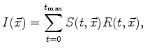
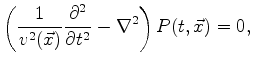
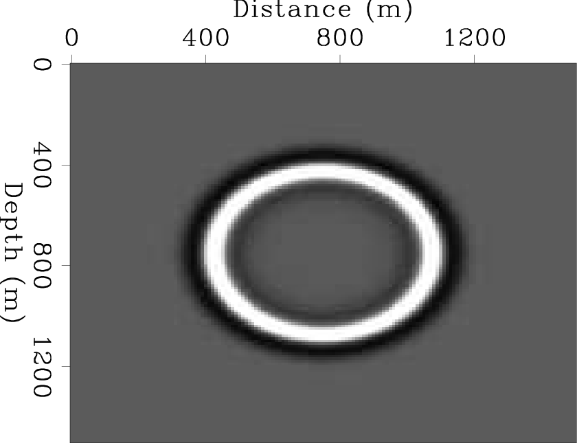
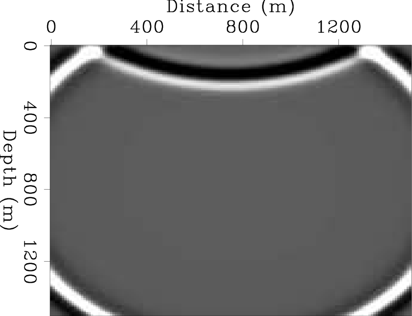
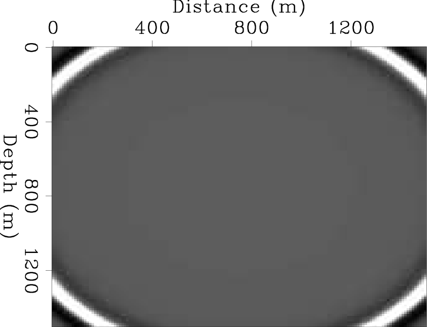
To illustrate the wavefield extrapolation used, Figures 1(a) and 1(b) show an extrapolated wavefield in a constant-velocity model with a reflecting top boundary, whereas Figures 1(c) and 1(d) show an extrapolated wavefield in the same model with an absorbing top boundary instead. The extrapolation using such an absorbing top boundary was used to generate seismic data without surface-related multiples (SRM).

wvfld0-mult1,wvfld0-mult2,wvfld0-nomult1,wvfld0-nomult2
Figure 1. Wavefield snapshots illustrate the wavefield extrapolation used in this paper. (a) and (b) show snapshots from a single modeling experiment with a reflecting top boundary at 0.25 and 0.55 seconds, respectively. (c) and (d) show snapshots from a single modeling experiment with a nonreflecting top boundary at 0.25 and 0.55 seconds, respectively.

Reverse-time migration using wavefield decomposition