 |
 |
 |
 | Wave-equation inversion of time-lapse seismic data sets |  |
![[pdf]](icons/pdf.png) |
Next: Bibliography
Up: APPENDIX A
Previous: Joint Inversion of Multiple
Because in the JMI formulation, the models are completely decoupled, they can be regularized by minimizing the norm
![\begin{displaymath}\begin{array}{ccc} \left \vert\left\vert \left [ \begin{array...
...rray} \right ] \right \vert \right \vert \approx 0 \end{array},\end{displaymath}](img117.png) |
(A-32) |
where
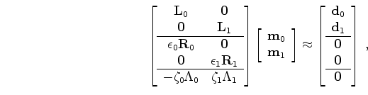 is the spatial regularization operator and
 the spatial regularization parameter for survey
  .
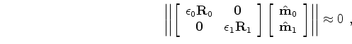
To add any temporal regularization, we need to warp the inverted monitor images to the baseline and then apply temporal constraints
or we can regularize the time-lapse image directly by minimizing the norm:
.
To add any temporal regularization, we need to warp the inverted monitor images to the baseline and then apply temporal constraints
or we can regularize the time-lapse image directly by minimizing the norm:
![\begin{displaymath}\begin{array}{ccc} \left \vert\left\vert \left [ \begin{array...
...rray} \right ] \right \vert \right \vert \approx 0 \end{array},\end{displaymath}](img120.png) |
(A-33) |
where
 is the temporal regularization operator and
  is the regularization parameter.
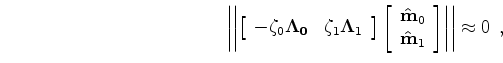
Therefore the full regularized inversion requires a minimization of the norm:
is the regularization parameter.
Therefore the full regularized inversion requires a minimization of the norm:
![\begin{displaymath}\begin{array}{ccc} \left \vert\left\vert \left [ \begin{array...
...rray} \right ] \right \vert \right \vert \approx 0 \end{array},\end{displaymath}](img123.png) |
(A-34) |
which leads to the image-space problem
![\begin{displaymath}\begin{array}{c} \left [ \begin{array}{ccc} {\bf H }_{0} & {\...
...\\ \hline {\bf0} \\ {\bf0} \\ \end{array} \right ], \end{array}\end{displaymath}](img124.png) |
(A-35) |
where
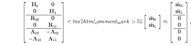 and
and
 are the spatial and temporal constraints, respectively.
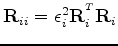
If the monitor has been aligned to the baseline, then we can impose the spatial regularization by minimizing
|
(A-36) |
and the temporal regularization by minimizing
|
(A-37) |
where
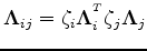 and
and
 are defined with respect to the baseline-aligned monitor image.
If the time-lapse image at the baseline position, the regularized image-space inversion problem is given by
are defined with respect to the baseline-aligned monitor image.
If the time-lapse image at the baseline position, the regularized image-space inversion problem is given by
![\begin{displaymath}\begin{array}{c} \left [ \begin{array}{ccc} {\bf H }_{0} & {\...
...\\ \hline {\bf0} \\ {\bf0} \\ \end{array} \right ], \end{array}\end{displaymath}](img26.png) |
(A-38) |
where the superscript  denotes that the operators and images are referenced to the baseline position.
Note that in the simplest case, where the temporal regularization is a difference operator equation A-33 becomes
denotes that the operators and images are referenced to the baseline position.
Note that in the simplest case, where the temporal regularization is a difference operator equation A-33 becomes
![\begin{displaymath}\begin{array}{ccc} \left \vert\left\vert \zeta \left [ \begin...
...rray} \right ] \right \vert \right \vert \approx 0 \end{array},\end{displaymath}](img130.png) |
(A-39) |
and for the baseline-aligned images, the temporal constraint in equation A-37 becomes
![\begin{displaymath}\begin{array}{ccc} \left \vert\left\vert \zeta \left [ \begin...
...rray} \right ] \right \vert \right \vert \approx 0 \end{array}.\end{displaymath}](img131.png) |
(A-40) |
|
|
|
|
| Wave-equation inversion of time-lapse seismic data sets | |
|
Next: Bibliography
Up: APPENDIX A
Previous: Joint Inversion of Multiple
2011-05-24